Chapter 7, part 4 of 6: trinomial trees
Welcome back, and I hope you all had a good Easter.
A few things happened in the QuantLib world during the past couple of weeks. First, a couple of blogs started publishing QuantLib-related posts: one by Matthias Groncki and another by Gouthaman Balaraman. They both look interesting (and they both use IPython notebooks, which I like, too).
Then, Klaus Spanderen started playing with Adjoint Algorithmic Differentiation, thus joining the already impressive roster of people working on it.
Finally, Jayanth R. Varma and Vineet Virmani from the Indian Institute of Management Ahmedabad have published a working paper that introduces QuantLib for teaching derivative pricing. We had little feedback from academia so far, so I was especially glad to hear from them (and if you, too, use QuantLib in the classroom, drop me a line.)
This week’s content is the fourth part of the series on the tree framework that started in this post. And of course, a reminder: you’re still in time for an early-bird discount on my next course. Details are at this link.
Follow me on Twitter if you want to be notified of new posts, or add me to your circles, or subscribe via RSS: the buttons for that are in the footer. Also, make sure to check my Training page.
Trinomial trees
In last post, I described binomial trees. As you might remember, they had a rather regular structure which allows one to implement them as just calculations on indices.
Trinomial trees are implemented as different beasts entirely, and have a lot more leeway in connecting nodes. The way they’re built (which is explained in greater detail in Brigo and Mercurio [1]) is sketched in the figure below: on each level in the tree, nodes are placed at an equal distance between them based on a center node with the same underlying value as the root of the tree; in the figure, the center nodes are \( A_3 \) and \( B_3 \), placed on the same vertical line. As you can see, the distance can be different on each level.
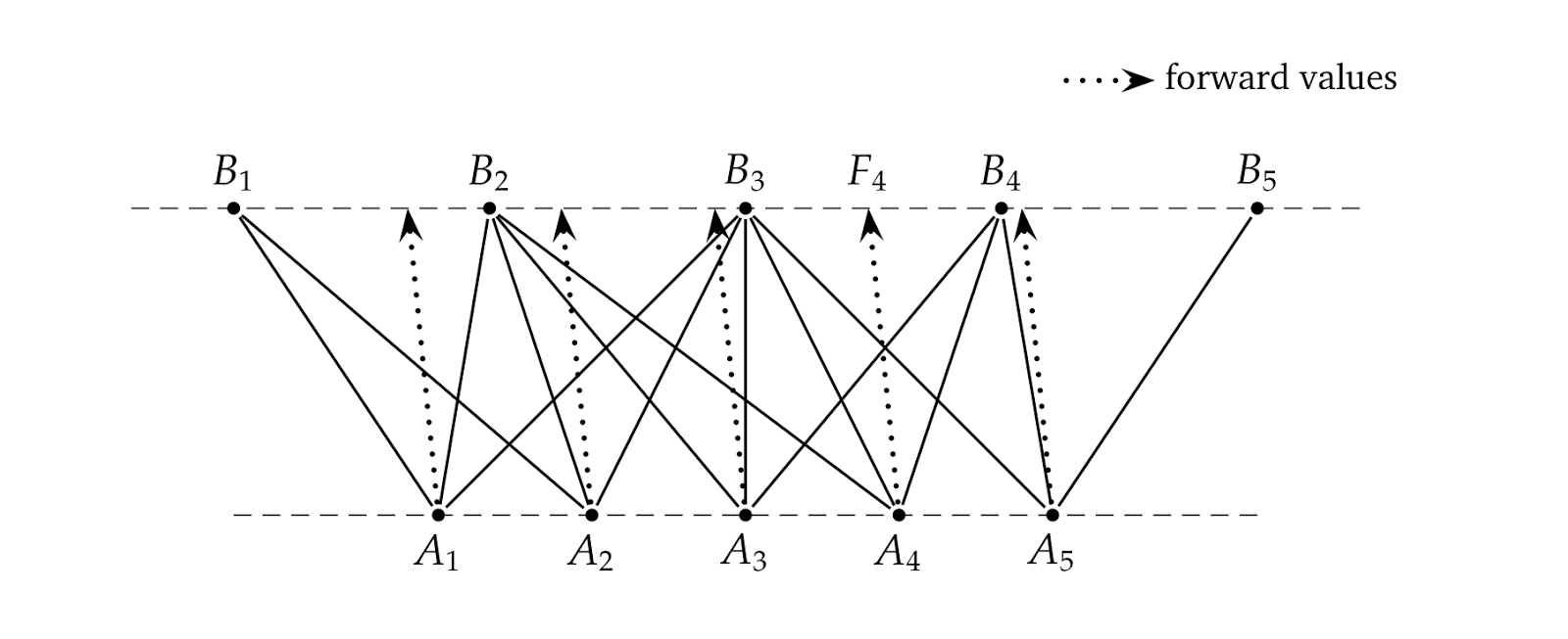
Once the nodes are in place, we build the links between them. Each node on a level corresponds, of course, to an underlying value \( x \) at the given time \( t \). From each of them, the process gives us the expectation value for the next time conditional to starting from \( (x, t) \); this is represented by the dotted lines. For each forward value, we determine the node which is closest and use that node for the middle branch. For instance, let’s look at the node \( A_4 \) in the figure. The dynamics of the underlying gives us a forward value corresponding to the point \( F_4 \) on the next level, which is closest to the node \( B_3 \). Therefore, \( A_4 \) branches out to \( B_3 \) in the middle and to its nearest siblings \( B_2 \) on the left and \( B_4 \) on the right.
As you see from the figure, it can well happen that two nodes on one level have forward values which are closest to the same node on the next level; see, for instance, nodes \( A_3 \) and \( A_4 \) going both to \( B_3 \) in the middle. This means that, while it’s guaranteed by construction that three branches start from each node, there’s no telling beforehand how many branches go to a given node; here we range from \( B_5 \) being the end node of just one branch to \( B_3 \) being the end node of five. There is also no telling how many nodes we’ll need at each level: in this case, five \( B \) nodes are enough to receive all the branches starting from five \( A \) nodes, but depending on the dynamics of the process we might have needed more nodes or fewer (you can try it: modify the distances in the figure and see what happens).
The logic I just described is implemented by QuantLib in the
TrinomialTree class, shown in the listing below.
    class TrinomialTree : public Tree<TrinomialTree> {
        class Branching;
      public:
        enum Branches { branches = 3 };
        TrinomialTree(
               const boost::shared_ptr<StochasticProcess1D>& process,
               const TimeGrid& timeGrid,
               bool isPositive = false);
        Real dx(Size i) const;
        const TimeGrid& timeGrid() const;
        Size size(Size i) const  {
            return i==0 ? 1 : branchings_[i-1].size();
        }
        Size descendant(Size i, Size index, Size branch) const;
        Real probability(Size i, Size index, Size branch) const;
        Real underlying(Size i, Size index) const {
            return i==0 ? x0_;
                x0_ + (branchings_[i-1].jMin() + index)*dx(i);
        }
      protected:
        std::vector<Branching> branchings_;
        Real x0_;
        std::vector<Real> dx_;
        TimeGrid timeGrid_;
    };
Its constructor takes a one-dimensional process, a time grid specifying the times corresponding to each level of the tree (which don’t need to be at regular intervals) and a boolean flag which, if set, constrains the underlying variable to be positive.
I’ll get to the construction in a minute, but first I need to show how
the information is stored; that is, I need to describe the inner
Branching class, shown in the next listing. Each instance of the
class stores the information for one level of the tree; e.g., one such
instance could encode the figure shown above (to which I’ll keep
referring).
    class TrinomialTree::Branching {
      public:
        Branching()
        : probs_(3), jMin_(QL_MAX_INTEGER), jMax_(QL_MIN_INTEGER) {}
        Size size() const {
            return jMax_ - jMin_ + 1;
        }
        Size descendant(Size i, Size branch) const {
            return k_[i] - jMin_ + branch - 1;
        }
        Real probability(Size i, Size branch) const {
            return probs_[branch][i];
        }
        Integer jMin() const;
        Integer jMax() const;
        void add(Integer k, Real p1, Real p2, Real p3) {
            k_.push_back(k);
            probs_[0].push_back(p1);
            probs_[1].push_back(p2);
            probs_[2].push_back(p3);

            jMin_ = std::min(jMin_, k-1);
            jMax_ = std::max(jMax_, k+1);
        }
      private:
        std::vector<Integer> k_;
        std::vector<std::vector<Real> > probs_;
        Integer jMin_, jMax_;
    };
As I mentioned, nodes are placed based on a center node corresponding
to the initial value of the underlying. That’s the only available
reference point, since we don’t know how many nodes we’ll use on
either side. Therefore, the Branching class uses an index system
that assigns the index \( j=0 \) to the center node and works
outwards from there. For instance, on the lower level in the figure
we’d have \( j=0 \) for \( A_3 \), \( j=1 \) for \( A_4 \),
\( j=-1 \) for \( A_2 \) and so on; on the upper level, we’d start
from \( j=0 \) for \( B_3 \). These indexes will have to be
translated to those used by the tree interface, that start at \( 0
\) for the leftmost node (\( A_1 \) in the figure).
To hold the tree information, the class declares as data members a vector of integers, storing for each lower-level node the index (in the branching system) of the corresponding mid-branch node on the upper level (there’s no need to store the indexes of the left-branch and right-branch nodes, as they are always the neighbors of the mid-branch one); three vectors, declared for convenience of access as a vector of vectors, storing the probabilities for each of the three branches; and two integers storing the minimum and maximum node index used on the upper level (again, in the branching system).
Implementing the tree interface requires some care with the several
indexes we need to juggle. For instance, let’s go back to
TrinomialTree and look at the size method. It must return the
number of nodes at level \( i \); and since each branching holds
information on the nodes of its upper level, the correct figure must
be retrieved branchings_[i-1] (except for the case \( i=0 \), for
which the result is \( 0 \) by construction). To allow this, the
Branching class provides a size method that returns the number of
points on the upper level; since jMin_ and jMax_ store the indexes
of the leftmost and rightmost node, respectively, the number to return
is jMax_-jMin_+1. In the figure, indexes go from \( -2 \) to \( 2
\) (corresponding to \( B_1 \) and \( B_5 \)) yielding \( 5 \)
as the number of nodes.
The descendant and probability methods of the tree both call
corresponding methods in the Branching class. The first returns the
descendant of the \( i \)-th lower-level node on the given branch
(specified as \( 0 \), \( 1 \) or \( 2 \) for the left, mid and
right branch, respectively). To do so, it first retrieves the index
\( k \) of the mid-branch node in the internal index system; then it
subtracts jMin, which transforms it in the corresponding external
index; and finally takes the branch into account by adding branch-1
(that is, \( -1 \), \( 0 \) or \( 1 \) for left, mid and right
branch). The probability method is easy enough: it selects the
correct vector based on the branch and returns the probability for the
\( i \)-th node. Since the vector indexes are zero-based, no
conversion is needed.
Finally, the underlying method is implemented by TrinomialTree
directly, since the branching doesn’t store the relevant process
information. The Branching class only needs to provide an inspector
jMin, which the tree uses to determine the offset of the leftmost
node from the center; it also provides a jMax inspector, as well as
an add method which is used to build the branching. Such method
should probably be called push_back instead; it takes the data for a
single node (that is, mid-branch index and probabilities), adds them
to the back of the corresponding vectors, and updates the information
on the minimum and maximum indexes.
What remains now is for me to show (with the help of the listing below
and, again, of the diagram at the beginning) how a TrinomialTree
instance is built.
    TrinomialTree::TrinomialTree(
               const boost::shared_ptr<StochasticProcess1D>& process,
               const TimeGrid& timeGrid,
               bool isPositive)
    : Tree<TrinomialTree>(timeGrid.size()), dx_(1, 0.0),
      timeGrid_(timeGrid) {
        x0_ = process->x0();
        Size nTimeSteps = timeGrid.size() - 1;
        Integer jMin = 0, jMax = 0;

        for (Size i=0; i<nTimeSteps; i++) {
            Time t = timeGrid[i];
            Time dt = timeGrid.dt(i);

            Real v2 = process->variance(t, 0.0, dt);
            Volatility v = std::sqrt(v2);
            dx_.push_back(v*std::sqrt(3.0));

            Branching branching;
            for (Integer j=jMin; j<=jMax; j++) {
                Real x = x0_ + j*dx_[i];
                Real f = process->expectation(t, x, dt);
                Integer k = std::floor((f-x0_)/dx_[i+1] + 0.5);

                if (isPositive)
                    while (x0_+(k-1)*dx_[i+1]<=0)
                        k++;

                Real e = f - (x0_ + k*dx_[i+1]);
                Real e2 = e*e, e3 = e*std::sqrt(3.0);

                Real p1 = (1.0 + e2/v2 - e3/v)/6.0;
                Real p2 = (2.0 - e2/v2)/3.0;
                Real p3 = (1.0 + e2/v2 + e3/v)/6.0;

                branching.add(k, p1, p2, p3);
            }
            branchings_.push_back(branching);
            jMin = branching.jMin();
            jMax = branching.jMax();
        }
    }
The constructor takes the stochastic process for the underlying
variable, a time grid, and a boolean flag. The number of times in the
grid corresponds to the number of levels in the tree, so it is passed
to the base Tree constructor; also, the time grid is stored and a
vector dx_, which will store the distances between nodes at the each
level, is initialized. The first level has just one node, so there’s
no corresponding distance to speak of; thus, the first element of the
vector is just set to \( 0 \). Other preparations include storing
the initial value x0_ of the underlying and the number of steps; and
finally, declaring two variables jMin and jMax to hold the minimum
and maximum node index. At the initial level, they both equal \( 0
\).
After this introduction, the tree is built recursively from one level
to the next. For each step, we take the initial time t and the time
step dt from the time grid. They’re used as input to retrieve the
variance of the process over the step, which is assumed to be
independent of the value of the underlying (as for binomial trees, we
have no way to enforce this). Based on the variance, we calculate the
distance to be used at the next level and store it in the dx_ vector
(the value of \( \sqrt{3} \) times the variance is suggested by Hull
and White as resulting in best stability) and after this, we finally
build a Branching instance.
To visualize the process, let’s refer again to the figure. The code
cycles over the nodes on the lower level, whose indexes range between
the current values of jMin and jMax: in our case, that’s \( -2
\) for \( A_1 \) and \( 2 \) for \( A_5 \). For each node, we
can calculate the underlying value x from the initial value x0_,
the index j, and the distance dx_[i] between the nodes. From x,
the process can give us the forward value f of the variable after
dt; and having just calculated the distance dx_[i+1] between nodes
on the upper level, we can find the index k of the node closest to
f. As usual, k is an internal index; for the node \( A_4 \) in
the figure, whose forward value is \( F_4 \), the index k would be
\( 0 \) corresponding to the center node \( B_3 \).
If the boolean flag isPositive is true, we have to make sure that no
node corresponds to a negative or null value of the underlying;
therefore, we check the value at the left target node (that would be
the one with index k-1, since k is the index of the middle one)
and if it’s not positive, we increase k and repeat until the desired
condition holds. In the figure, if the underlying were negative at
node \( B_1 \) then node \( A_1 \) would branch to \( B_2 \),
\( B_3 \) and \( B_4 \) instead.
Finally, we calculate the three transition probabilities p1, p2
and p3 (the formulas are derived in [1]) and store them in the
current Branching instance together with k. When all the nodes are
processed, we store the branching and update the values of jMin and
jMax so that they range over the nodes on the upper level; the new
values will be used for the next step of the main for loop (the one
over time steps) in which the current upper level will become the
lower level.
Bibliography
[1] D. Brigo and F. Mercurio, Interest Rate Models — Theory and Practice, 2nd edition. Springer, 2006.