A QuantLib-Python companion for the Ametrano-Bianchetti paper
Hello everybody.
It recently occurred to me that it’s 10 years since the paper by F. M. Ametrano and M. Bianchetti, Everything You Always Wanted to Know About Multiple Interest Rate Curve Bootstrapping but Were Afraid to Ask, was published on SSRN. Given the nice, round anniversary, I’m publishing here a companion Jupyter notebook that reproduces the calculations in the paper. Previously, this notebook was only available by buying the Quantlib Python Cookbook. Hint: there’s more where this came from.
Here we go. Grab something to drink, it’s a long read. Oh, and you can download the notebook if you want to play with it.
Subscribe to my Substack to receive my posts in your inbox, or follow me on Twitter or LinkedIn if you want to be notified of new posts, or subscribe via RSS if you’re the tech type: the buttons for all that are in the footer. Also, I’m available for training, both online and (when possible) on-site: visit my Training page for more information.
An Ametrano-Bianchetti companion
In this notebook, I’ll reproduce the results of the paper by F. M. Ametrano and M. Bianchetti, Everything You Always Wanted to Know About Multiple Interest Rate Curve Bootstrapping but Were Afraid to Ask (April 2013).
I won’t follow strictly the structure of the paper which, as usual for this kind of work, starts by laying down a theoretical framework. This notebook is meant to be read side to side with it, so there’s no reason for to repeat that part. Instead, I’ll jump ahead to the bootstrapping example in section 5 of the paper; and, as we proceed and add features in the code, I’ll refer to the corresponding earlier sections and subsections.
Without further ado, let’s import a few modules we’ll need (including, of course, QuantLib) and set the global evaluation date to the reference date used in the paper.
import math
import numpy as np
from matplotlib import pyplot as plt
from matplotlib.ticker import PercentFormatter
from datetime import date
import QuantLib as ql
today = ql.Date(11, ql.December, 2012)
ql.Settings.instance().evaluationDate = today
Eonia yield curve
Following the sequence of section 5, we start by bootstrapping the Eonia curve. There’s a reason for that; this curve is going to be used as a discount curve in the bootstrap of all the other forecast curves. Our aim is to reproduce the two plots in figure 26.
We start by instantiating helpers for all the rates used in the bootstrapping process, as reported in figure (table?) 25 of the paper.
The first three instruments are three 1-day deposit that give us
discounting between today and the day after spot. They are modeled by
three instances of the DepositRateHelper class, with a tenor of 1 day
and a number of fixing days going from 0 (for the deposit starting
today) to 2 (for the deposit starting on the spot date).
Note that these helpers, and the library in general, requires rates to be in decimal format; that is, a 1% rate must be entered as 0.01. Therefore, we need to divide the quotes in figure 25 by 100.
helpers = [
    ql.DepositRateHelper(
        ql.QuoteHandle(ql.SimpleQuote(rate / 100)),
        ql.Period(1, ql.Days),
        fixingDays,
        ql.TARGET(),
        ql.Following,
        False,
        ql.Actual360(),
    )
    for rate, fixingDays in [(0.04, 0), (0.04, 1), (0.04, 2)]
]
Then, we have a series of OIS quotes for the first month. They are
modeled by instances of the OISRateHelper class with varying tenors.
They also require an instance of the Eonia class, which doesn’t need a
forecast curve and can be shared between the helpers.
Another note: there are examples floating around the web (and, until
recently, in our own examples) in which the index passed to the helpers
is instantiated by passing it a RelinkableYieldTermStructureHandle,
and the handle is later linked to the curve we’re bootstrapping. Don’t
do that. It will create a cycle between objects and result in a memory
leak. When we have the curve, we’ll use it to create another instance of
the index.
eonia = ql.Eonia()
helpers += [
    ql.OISRateHelper(
        2, ql.Period(*tenor), ql.QuoteHandle(ql.SimpleQuote(rate / 100)), eonia
    )
    for rate, tenor in [
        (0.070, (1, ql.Weeks)),
        (0.069, (2, ql.Weeks)),
        (0.078, (3, ql.Weeks)),
        (0.074, (1, ql.Months)),
    ]
]
Next, five OIS forwards on ECB dates. For these, we need to instantiate
the DatedOISRateHelper class and specify start and end dates
explicitly.
helpers += [
    ql.DatedOISRateHelper(
        start_date, end_date, ql.QuoteHandle(ql.SimpleQuote(rate / 100)), eonia
    )
    for rate, start_date, end_date in [
        (0.046, ql.Date(16, ql.January, 2013), ql.Date(13, ql.February, 2013)),
        (0.016, ql.Date(13, ql.February, 2013), ql.Date(13, ql.March, 2013)),
        (-0.007, ql.Date(13, ql.March, 2013), ql.Date(10, ql.April, 2013)),
        (-0.013, ql.Date(10, ql.April, 2013), ql.Date(8, ql.May, 2013)),
        (-0.014, ql.Date(8, ql.May, 2013), ql.Date(12, ql.June, 2013)),
    ]
]
Finally, we add OIS quotes up to 30 years. These have a rolling
maturity, so we go back to the OisRateHelper class.
helpers += [
    ql.OISRateHelper(
        2, ql.Period(*tenor), ql.QuoteHandle(ql.SimpleQuote(rate / 100)), eonia
    )
    for rate, tenor in [
        (0.002, (15, ql.Months)),
        (0.008, (18, ql.Months)),
        (0.021, (21, ql.Months)),
        (0.036, (2, ql.Years)),
        (0.127, (3, ql.Years)),
        (0.274, (4, ql.Years)),
        (0.456, (5, ql.Years)),
        (0.647, (6, ql.Years)),
        (0.827, (7, ql.Years)),
        (0.996, (8, ql.Years)),
        (1.147, (9, ql.Years)),
        (1.280, (10, ql.Years)),
        (1.404, (11, ql.Years)),
        (1.516, (12, ql.Years)),
        (1.764, (15, ql.Years)),
        (1.939, (20, ql.Years)),
        (2.003, (25, ql.Years)),
        (2.038, (30, ql.Years)),
    ]
]
The curve is an instance of PiecewiseLogCubicDiscount (corresponding
to the PiecewiseYieldCurve<Discount,LogCubic> class in C++); the
argument for this choice is made in section 4.5 of the paper. We let the
reference date of the curve move with the global evaluation date, by
specifying it as 0 days after the latter on the TARGET calendar.
The day counter chosen is not of much consequence, as it is only used internally to convert dates into times. As mentioned in section 4.2, a additive day-count convention is to be preferred; that is, one for which, given three dates $d_1$, $d_2$ and $d_3$,
\[\tau(d_1, d_3) = \tau(d_1, d_2) + \tau(d_2, d_3)\]In practice, this usually means the Act/360 or Act/365 conventions.
Also, we enable extrapolation beyond the maturity of the last helper; that is mostly for convenience as we retrieve rates to plot the curve near its far end.
eonia_curve_c = ql.PiecewiseLogCubicDiscount(
    0, ql.TARGET(), helpers, ql.Actual365Fixed()
)
eonia_curve_c.enableExtrapolation()
To compare the curve with the one shown in figure 26 of the paper, we can retrieve daily overnight rates over its first two years and plot them:
today = eonia_curve_c.referenceDate()
end = today + ql.Period(2, ql.Years)
dates = [
    ql.Date(serial)
    for serial in range(today.serialNumber(), end.serialNumber() + 1)
]
rates_c = [
    eonia_curve_c.forwardRate(
        d, ql.TARGET().advance(d, 1, ql.Days), ql.Actual360(), ql.Simple
    ).rate()
    for d in dates
]

ax = plt.figure(figsize=(9, 6)).add_subplot(1, 1, 1)
ax.axhline(0.0, linewidth=1, color="black")
ax.set_xlim(min(dates).to_date(), max(dates).to_date())
ax.yaxis.set_major_formatter(PercentFormatter(1.0))
ax.plot_date([d.to_date() for d in dates], rates_c, "-");
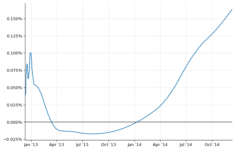
However, we still have work to do. Out plot above shows a rather large bump at the end of 2012 which is not present in the paper. To remove it, we need to model properly the turn-of-year effect.
Turn-of-year jumps
As explained in section 4.8 of the paper, the turn-of-year effect is a
jump in interest rates due to an increased demand for liquidity at the
end of the year. The jump is embedded in any quoted rates that straddle
the end of the year, and must be treated separately; the
YieldTermStructure class allows this by taking any number of jumps,
modeled as additional discount factors, and applying them at the
specified dates.
Our current problem, however, is to estimate the size of the jump. To
simplify analysis, we turn to flat forward rates instead of log-cubic
discounts; thus, we instantiate a PiecewiseFlatForward curve
(corresponding to PiecewiseYieldCurve<ForwardRate,BackwardFlat> in
C++).
eonia_curve_ff = ql.PiecewiseFlatForward(
    0, ql.TARGET(), helpers, ql.Actual365Fixed()
)
eonia_curve_ff.enableExtrapolation()
To show the jump more clearly, I’ll restrict the plot to the first 6 months:
end = today + ql.Period(6, ql.Months)
dates = [
    ql.Date(serial)
    for serial in range(today.serialNumber(), end.serialNumber() + 1)
]
rates_ff = [
    eonia_curve_ff.forwardRate(
        d, ql.TARGET().advance(d, 1, ql.Days), ql.Actual360(), ql.Simple
    ).rate()
    for d in dates
]

ax = plt.figure(figsize=(9, 6)).add_subplot(1, 1, 1)
ax.axhline(0.0, linewidth=1, color="black")
ax.set_xlim(min(dates).to_date(), max(dates).to_date())
ax.yaxis.set_major_formatter(PercentFormatter(1.0))
ax.plot_date([d.to_date() for d in dates], rates_ff, "-");
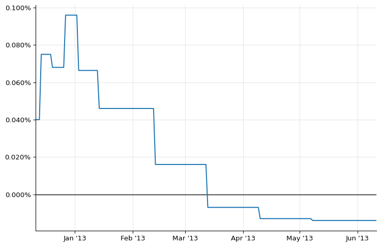
As we see, the forward ending at the beginning of January 2013 is out of line. In order to estimate the jump, we need to estimate a “clean” forward that doesn’t include it.
A possible estimate (although not the only one) can be obtained by interpolating the forwards around the one we want to replace. To do so, we extract the values of the forwards rates and their corresponding dates.
nodes = list(eonia_curve_ff.nodes())
If we look at the first few nodes, we can clearly see that the seventh (the one for January 2013) is out of line.
nodes[:9]
[(Date(11,12,2012), 0.00040555533025081675),
 (Date(12,12,2012), 0.00040555533025081675),
 (Date(13,12,2012), 0.00040555533047721286),
 (Date(14,12,2012), 0.00040555533047721286),
 (Date(20,12,2012), 0.0007604110692568178),
 (Date(27,12,2012), 0.0006894305026004767),
 (Date(3,1,2013), 0.0009732981324671213),
 (Date(14,1,2013), 0.0006728161005748453),
 (Date(13,2,2013), 0.00046638054590758754)]
To create a curve that doesn’t include the jump, we replace the relevant forward rate with a simple average of the ones that precede and follow…
nodes[6] = (nodes[6][0], (nodes[5][1] + nodes[7][1]) / 2.0)
nodes[:9]
[(Date(11,12,2012), 0.00040555533025081675),
 (Date(12,12,2012), 0.00040555533025081675),
 (Date(13,12,2012), 0.00040555533047721286),
 (Date(14,12,2012), 0.00040555533047721286),
 (Date(20,12,2012), 0.0007604110692568178),
 (Date(27,12,2012), 0.0006894305026004767),
 (Date(3,1,2013), 0.000681123301587661),
 (Date(14,1,2013), 0.0006728161005748453),
 (Date(13,2,2013), 0.00046638054590758754)]
…and instantiate a ForwardCurve with the modified nodes.
temp_dates, temp_rates = zip(*nodes)
temp_curve = ql.ForwardCurve(
    temp_dates, temp_rates, eonia_curve_ff.dayCounter()
)
For illustration, we can extract daily overnight nodes from the doctored curve and plot them alongside the old ones:
temp_rates = [
    temp_curve.forwardRate(
        d, ql.TARGET().advance(d, 1, ql.Days), ql.Actual360(), ql.Simple
    ).rate()
    for d in dates
]

ax = plt.figure(figsize=(9, 6)).add_subplot(1, 1, 1)
ax.axhline(0.0, linewidth=1, color="black")
ax.set_xlim(min(dates).to_date(), max(dates).to_date())
ax.yaxis.set_major_formatter(PercentFormatter(1.0))
ax.plot_date(
    [d.to_date() for d in dates], temp_rates, "-", label="doctored curve"
)
ax.plot_date(
    [d.to_date() for d in dates], rates_ff, "--", label="original curve"
)
ax.legend();
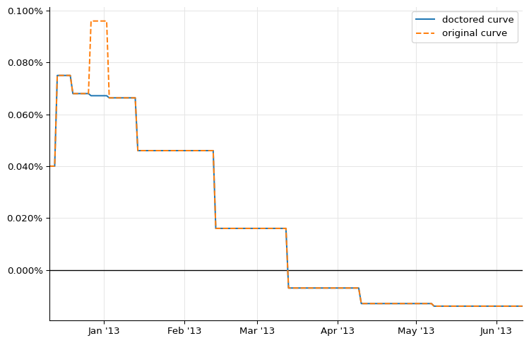
Now we can estimate the size of the jump. As the paper hints, it’s more an art than a science. I’ve been able to reproduce fairly closely the results of the paper by extracting from both curves the forward rate over the two weeks around the end of the year:
d1 = ql.Date(31, ql.December, 2012) - ql.Period(1, ql.Weeks)
d2 = ql.Date(31, ql.December, 2012) + ql.Period(1, ql.Weeks)
F = eonia_curve_ff.forwardRate(d1, d2, ql.Actual360(), ql.Simple)
F_1 = temp_curve.forwardRate(d1, d2, ql.Actual360(), ql.Simple)
print(F)
print(F_1)
0.081531 % Actual/360 simple compounding
0.067122 % Actual/360 simple compounding
We want to attribute the whole jump to the last day of the year, so we rescale it according to
\[(F-F_1) \cdot t_{12} = J \cdot t_J\]where $t_{12}$ is the time between the two dates and $t_J$ is the time between the start and end date of the end-of-year overnight deposit. This gives us a jump close to the value of 10.2 basis points reported in the paper.
t12 = eonia_curve_ff.dayCounter().yearFraction(d1, d2)
t_j = eonia_curve_ff.dayCounter().yearFraction(
    ql.Date(31, ql.December, 2012), ql.Date(2, ql.January, 2013)
)
J = (F.rate() - F_1.rate()) * t12 / t_j
print(f"{J*100:.4} %")
0.1009 %
As I mentioned previously, the jump can be added to the curve as a corresponding discount factor $1/(1+J \cdot t_J)$ on the last day of the year. The information can be passed to the curve constructor, giving us a new instance:
B = 1.0 / (1.0 + J * t_j)
jumps = [ql.QuoteHandle(ql.SimpleQuote(B))]
jump_dates = [ql.Date(31, ql.December, 2012)]
eonia_curve_j = ql.PiecewiseFlatForward(
    0, ql.TARGET(), helpers, ql.Actual365Fixed(), jumps, jump_dates
)
Retrieving daily overnight rates from the new curve and plotting them, we can see the jump quite clearly:
rates_j = [
    eonia_curve_j.forwardRate(
        d, ql.TARGET().advance(d, 1, ql.Days), ql.Actual360(), ql.Simple
    ).rate()
    for d in dates
]

ax = plt.figure(figsize=(9, 6)).add_subplot(1, 1, 1)
ax.axhline(0.0, linewidth=1, color="black")
ax.set_xlim(min(dates).to_date(), max(dates).to_date())
ax.yaxis.set_major_formatter(PercentFormatter(1.0))
ax.plot_date([d.to_date() for d in dates], rates_ff, "-", label="without jump")
ax.plot_date([d.to_date() for d in dates], rates_j, "o", label="with jump")
ax.legend();
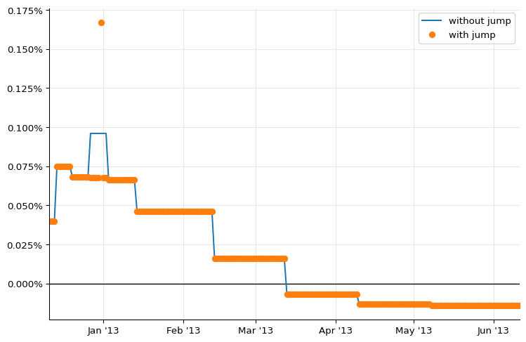
We can now go back to log-cubic discounts and add the jump.
eonia_curve = ql.PiecewiseLogCubicDiscount(
    0, ql.TARGET(), helpers, ql.Actual365Fixed(), jumps, jump_dates
)
eonia_curve.enableExtrapolation()
rates_c = [
    eonia_curve_c.forwardRate(
        d, ql.TARGET().advance(d, 1, ql.Days), ql.Actual360(), ql.Simple
    ).rate()
    for d in dates
]
rates = [
    eonia_curve.forwardRate(
        d, ql.TARGET().advance(d, 1, ql.Days), ql.Actual360(), ql.Simple
    ).rate()
    for d in dates
]

ax = plt.figure(figsize=(9, 6)).add_subplot(1, 1, 1)
ax.axhline(0.0, linewidth=1, color="black")
ax.set_xlim(min(dates).to_date(), max(dates).to_date())
ax.yaxis.set_major_formatter(PercentFormatter(1.0))
ax.plot_date([d.to_date() for d in dates], rates_c, "-", label="without jump")
ax.plot_date([d.to_date() for d in dates], rates, "o", label="with jump")
ax.legend();
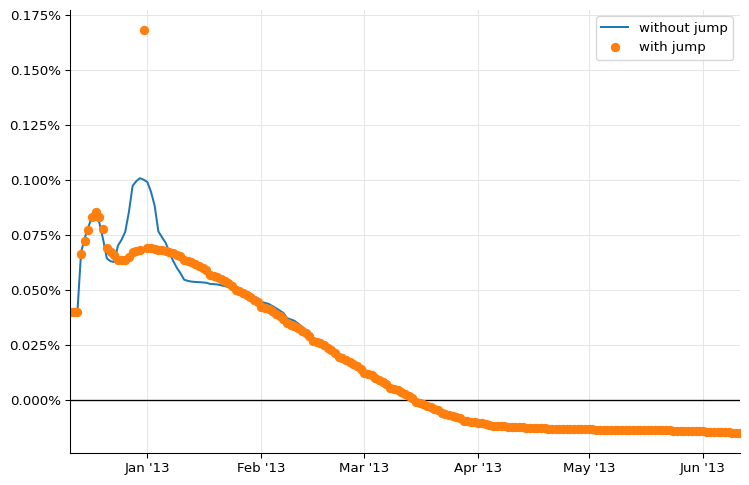
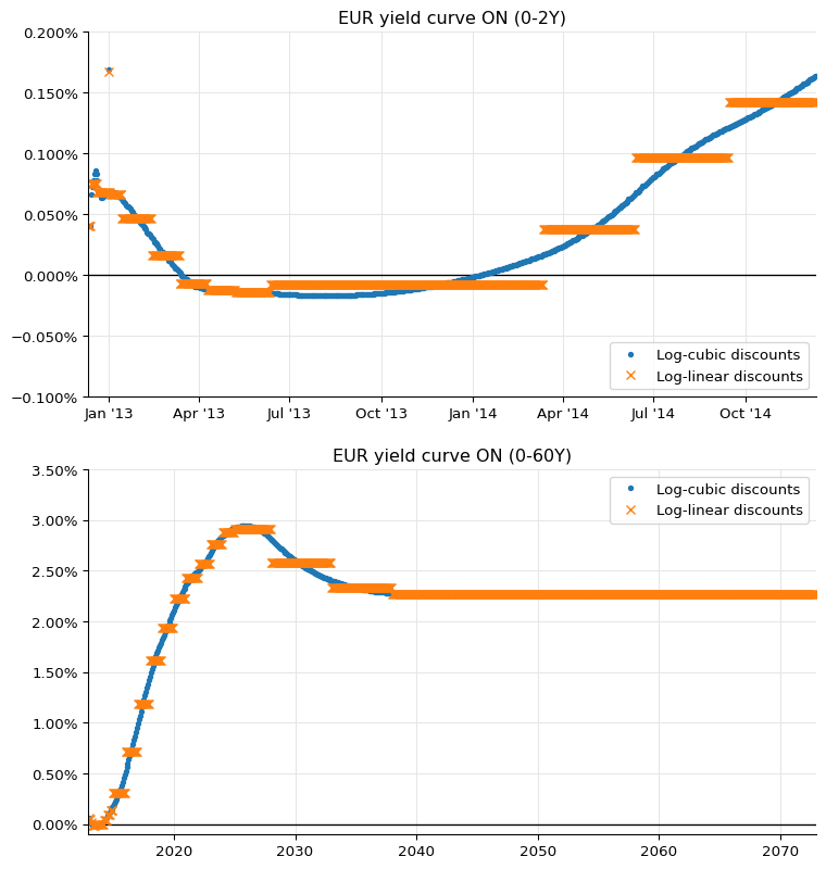
As you can see, the large bump is gone now. The two plots in figure 26 can be reproduced as follows (omitting the jump at the end of 2013 for brevity, and the flat forwards for clarity):
eonia_curve_2 = ql.PiecewiseLogLinearDiscount(
    0, ql.TARGET(), helpers, ql.Actual365Fixed(), jumps, jump_dates
)
eonia_curve_2.enableExtrapolation()
fig = plt.figure(figsize=(9, 10))

dates = [today + ql.Period(i, ql.Days) for i in range(0, 365 * 2 + 1)]
rates = [
    eonia_curve.forwardRate(
        d, ql.TARGET().advance(d, 1, ql.Days), ql.Actual360(), ql.Simple
    ).rate()
    for d in dates
]
rates_2 = [
    eonia_curve_2.forwardRate(
        d, ql.TARGET().advance(d, 1, ql.Days), ql.Actual360(), ql.Simple
    ).rate()
    for d in dates
]

ax1 = fig.add_subplot(2, 1, 1)
ax1.set_title("EUR yield curve ON (0-2Y)")
ax1.axhline(0.0, linewidth=1, color="black")
ax1.set_xlim(min(dates).to_date(), max(dates).to_date())
ax1.yaxis.set_major_formatter(PercentFormatter(1.0))
ax1.set_ylim(-0.001, 0.002)
ax1.plot_date(
    [d.to_date() for d in dates], rates, ".", label="Log-cubic discounts"
)
ax1.plot_date(
    [d.to_date() for d in dates], rates_2, "x", label="Log-linear discounts"
)
ax1.legend(loc="lower right")

dates = [today + ql.Period(i, ql.Months) for i in range(0, 12 * 60 + 1)]
rates = [
    eonia_curve.forwardRate(
        d, ql.TARGET().advance(d, 1, ql.Days), ql.Actual360(), ql.Simple
    ).rate()
    for d in dates
]
rates_2 = [
    eonia_curve_2.forwardRate(
        d, ql.TARGET().advance(d, 1, ql.Days), ql.Actual360(), ql.Simple
    ).rate()
    for d in dates
]

ax2 = fig.add_subplot(2, 1, 2)
ax2.set_title("EUR yield curve ON (0-60Y)")
ax2.axhline(0.0, linewidth=1, color="black")
ax2.set_xlim(min(dates).to_date(), max(dates).to_date())
ax2.yaxis.set_major_formatter(PercentFormatter(1.0))
ax2.set_ylim(-0.001, 0.035)
ax2.plot_date(
    [d.to_date() for d in dates], rates, ".", label="Log-cubic discounts"
)
ax2.plot_date(
    [d.to_date() for d in dates], rates_2, "x", label="Log-linear discounts"
)
ax2.legend(loc="upper right");
A final word of warning: as you saw, the estimate of the jumps is not an exact science, so it’s best to check it manually and not to leave it to an automated procedure.
Moreover, jumps might be present at the end of each month, as reported for instance in Paolo Mazzocchi’s presentation at the QuantLib User Meeting 2014. This, too, suggests particular care in building the Eonia curve.
6-months Euribor curve
As we’ll see, most of the Euribor curves for different tenors have their own quirks.
I’ll start from the 6-months Euribor curve, which is somewhat simpler due to having a number of quoted rates directly available for bootstrapping. The figure we want to reproduce is figure 32; the market data are in figure 31.
The first instrument used in the paper if the TOM 6-months FRA, which can be instantiated as a 6-months deposit with 3 fixing days; its rate (and those of all other FRAs) is retrieved from figure 6 in the paper.
helpers = [
    ql.DepositRateHelper(
        ql.QuoteHandle(ql.SimpleQuote(0.312 / 100)),
        ql.Period(6, ql.Months),
        3,
        ql.TARGET(),
        ql.Following,
        False,
        ql.Actual360(),
    )
]
Then comes a strip of 6-months FRA up to 2 years maturity. The
FraRateHelper class needs an instance of the corresponding index that,
again, we instantiate without passing it a handle.
euribor6m = ql.Euribor6M()
helpers += [
    ql.FraRateHelper(
        ql.QuoteHandle(ql.SimpleQuote(rate / 100)), start, euribor6m
    )
    for rate, start in [
        (0.293, 1),
        (0.272, 2),
        (0.260, 3),
        (0.256, 4),
        (0.252, 5),
        (0.248, 6),
        (0.254, 7),
        (0.261, 8),
        (0.267, 9),
        (0.279, 10),
        (0.291, 11),
        (0.303, 12),
        (0.318, 13),
        (0.335, 14),
        (0.352, 15),
        (0.371, 16),
        (0.389, 17),
        (0.409, 18),
    ]
]
Finally, we have a series of swap rates with maturities from 3 to 60
years, listed in figure 9. As the paper explains (see section 4.7), the
curve being bootstrapped will be used only for forecasting the 6-months
Euribor fixings paid by the floating leg; all the payments will be
discounted by means of the OIS curve. In the implementation, this is
done by wrapping the Eonia curve in a Handle and passing it as an
extra argument to the SwapRateHelper constructor.
discount_curve = ql.YieldTermStructureHandle(eonia_curve)
helpers += [
    ql.SwapRateHelper(
        ql.QuoteHandle(ql.SimpleQuote(rate / 100)),
        ql.Period(tenor, ql.Years),
        ql.TARGET(),
        ql.Annual,
        ql.Unadjusted,
        ql.Thirty360(ql.Thirty360.BondBasis),
        euribor6m,
        ql.QuoteHandle(),
        ql.Period(0, ql.Days),
        discount_curve,
    )
    for rate, tenor in [
        (0.424, 3),
        (0.576, 4),
        (0.762, 5),
        (0.954, 6),
        (1.135, 7),
        (1.303, 8),
        (1.452, 9),
        (1.584, 10),
        (1.809, 12),
        (2.037, 15),
        (2.187, 20),
        (2.234, 25),
        (2.256, 30),
        (2.295, 35),
        (2.348, 40),
        (2.421, 50),
        (2.463, 60),
    ]
]
This will give us a decent Euribor curve, that we can display by sampling 6-months forward rates at a number of dates.
euribor6m_curve = ql.PiecewiseLogCubicDiscount(
    2, ql.TARGET(), helpers, ql.Actual365Fixed()
)
euribor6m_curve.enableExtrapolation()
spot = euribor6m_curve.referenceDate()
dates = [spot + ql.Period(i, ql.Months) for i in range(0, 60 * 12 + 1)]
rates = [
    euribor6m_curve.forwardRate(
        d, euribor6m.maturityDate(d), ql.Actual360(), ql.Simple
    ).rate()
    for d in dates
]

ax = plt.figure(figsize=(9, 6)).add_subplot(1, 1, 1)
ax.axhline(0.0, linewidth=1, color="black")
ax.set_xlim(min(dates).to_date(), max(dates).to_date())
ax.yaxis.set_major_formatter(PercentFormatter(1.0))
ax.plot_date([d.to_date() for d in dates], rates, "-");
At the scale of the plot, this seems to work and to match figure 32 in the paper; but looking closely at the first part of the curve, you can see a glitch (some kind of dip) in the last part of 2014, when the FRA strip ends.
dates = [spot + ql.Period(i, ql.Weeks) for i in range(0, 52 * 4 + 1)]
rates = [
    euribor6m_curve.forwardRate(
        d, euribor6m.maturityDate(d), ql.Actual360(), ql.Simple
    ).rate()
    for d in dates
]

ax = plt.figure(figsize=(9, 6)).add_subplot(1, 1, 1)
ax.axhline(0.0, linewidth=1, color="black")
ax.set_xlim(min(dates).to_date(), max(dates).to_date())
ax.yaxis.set_major_formatter(PercentFormatter(1.0))
ax.plot_date([d.to_date() for d in dates], rates, "-")
ax.annotate(
    "",
    xy=(date(2014, 10, 1), 0.0055),
    xytext=(date(2014, 8, 1), 0.008),
    arrowprops=dict(arrowstyle="->"),
);
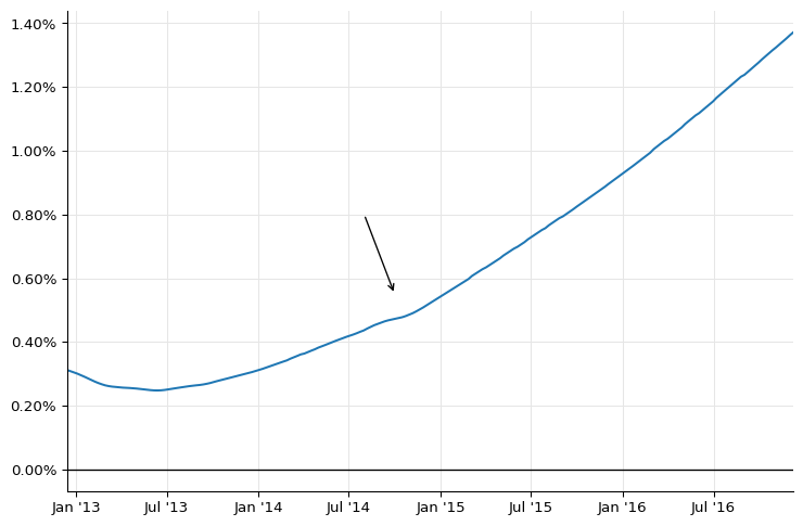
Synthetic deposits
In short, the reason is that the short end of the curve (which is required for pricing FRAs; for instance, the 1x7 FRA required the discount factor at 1 month from now) is extrapolated backwards from the first quoted pillar at 6 months and is not quite correct. This leads to oscillations as soon as the curve is out of the tight strip of FRA quotes.
One way to correct this is to add synthetic deposits with short tenors, as explained in section 4.4.2 of the paper. To begin with, let’s save the original curve to another variable for later comparison.
euribor6m_curve_0 = euribor6m_curve
As detailed in the paper, one can model the basis between the Euribor market quotes and the corresponding OIS-based rates as a polynomial; that is, following equation 88,
\[R_{x}(T_1,T_2) \tau(T_1,T_2) = R_{on}(T_1,T_2) \tau(T_1,T_2) + \Delta(T_1,T_2)\]In the paper, the expression for $\Delta(T_1,T_2)$ is given by equation 90, that is,
\[\Delta(T_1, T_2) = \alpha \cdot (T_2-T_1) + \frac{1}{2} \beta \cdot (T_2-T_1)^2 + \frac{1}{3} \gamma \cdot (T_2-T_1)^3 + \ldots\]However, the above leads to problems when trying to solve for more than one coefficient. Following a later formulation, I’ll express the instantaneous basis instead as
\[\delta(t) = \alpha + \beta \cdot t + \gamma \cdot t^2 + \ldots\]which leads to
\[\Delta(T_1, T_2) = \int_{T_1}^{T_2} \delta(t) = \alpha \cdot (T_2-T_1) + \frac{1}{2} \beta \cdot (T_2^2-T_1^2) + \frac{1}{3} \gamma \cdot (T_2^3-T_1^3) + \ldots\]Once the basis is known, we can calculate synthetic deposit rates $R(0,T)$ for any maturity $T$.
Depending on how many polynomial coefficients we want to determine, we’ll need a corresponding number of market quotes; by replacing their values and those of the OIS rates in equation 88 we can solve for $\alpha$, $\beta$ and any other coefficient.
For a constant polynomial, we’ll need one quote to determine $\alpha$; we can use the TOM 6-months deposit that the Euribor curve reprices exactly.
d = ql.TARGET().advance(spot, 1, ql.Days)
F_x = euribor6m_curve_0.forwardRate(
    d, ql.TARGET().advance(d, 6, ql.Months), ql.Actual360(), ql.Simple
).rate()
F_on = eonia_curve.forwardRate(
    d, ql.TARGET().advance(d, 6, ql.Months), ql.Actual360(), ql.Simple
).rate()
day_counter = euribor6m.dayCounter()
T_x = day_counter.yearFraction(d, ql.TARGET().advance(d, 6, ql.Months))
alpha = F_x - F_on
print(alpha)
0.0029492968598198548
From the basis, we can instantiate synthetic deposits for a number of maturities below 6 months…
synth_helpers = []
for n, units in [
    (1, ql.Days),
    (1, ql.Weeks),
    (2, ql.Weeks),
    (3, ql.Weeks),
    (1, ql.Months),
    (2, ql.Months),
    (3, ql.Months),
    (4, ql.Months),
    (5, ql.Months),
]:
    t = day_counter.yearFraction(spot, ql.TARGET().advance(spot, n, units))
    F_on = eonia_curve.forwardRate(
        spot, ql.TARGET().advance(spot, n, units), ql.Actual360(), ql.Simple
    ).rate()
    F = F_on + alpha
    print(f"{ql.Period(n, units)}: {F*100:.4} %")
    synth_helpers.append(
        ql.DepositRateHelper(
            ql.QuoteHandle(ql.SimpleQuote(F)),
            ql.Period(n, units),
            2,
            ql.TARGET(),
            ql.Following,
            False,
            ql.Actual360(),
        )
    )
1D: 0.3349 %
1W: 0.3649 %
2W: 0.3639 %
3W: 0.3729 %
1M: 0.3689 %
2M: 0.3559 %
3M: 0.3419 %
4M: 0.3272 %
5M: 0.3188 %
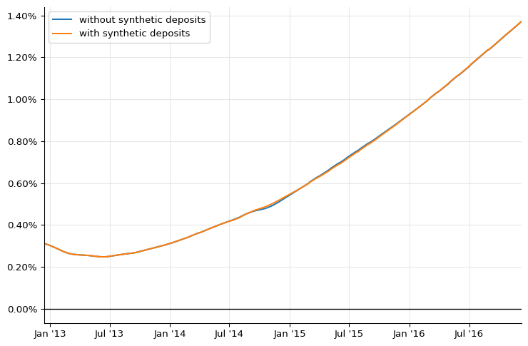
…after which we can create a new curve, which seems to have a smaller dip:
euribor6m_curve = ql.PiecewiseLogCubicDiscount(
    2, ql.TARGET(), helpers + synth_helpers, ql.Actual365Fixed()
)
euribor6m_curve.enableExtrapolation()
dates = [spot + ql.Period(i, ql.Weeks) for i in range(0, 52 * 4 + 1)]
rates_0 = [
    euribor6m_curve_0.forwardRate(
        d, euribor6m.maturityDate(d), ql.Actual360(), ql.Simple
    ).rate()
    for d in dates
]
rates = [
    euribor6m_curve.forwardRate(
        d, euribor6m.maturityDate(d), ql.Actual360(), ql.Simple
    ).rate()
    for d in dates
]

ax = plt.figure(figsize=(9, 6)).add_subplot(1, 1, 1)
ax.axhline(0.0, linewidth=1, color="black")
ax.set_xlim(min(dates).to_date(), max(dates).to_date())
ax.yaxis.set_major_formatter(PercentFormatter(1.0))
ax.plot_date(
    [d.to_date() for d in dates],
    rates_0,
    "-",
    label="without synthetic deposits",
)
ax.plot_date(
    [d.to_date() for d in dates], rates, "-", label="with synthetic deposits"
)
ax.legend();
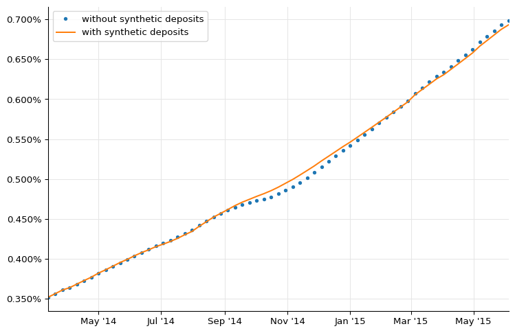
By choosing to sample at different dates, we can zoom into the affected area. The original curve is the dotted line; the new curve is the solid one.
dates = [spot + ql.Period(i, ql.Weeks) for i in range(65, 130)]
rates_0 = [
    euribor6m_curve_0.forwardRate(
        d, euribor6m.maturityDate(d), ql.Actual360(), ql.Simple
    ).rate()
    for d in dates
]
rates = [
    euribor6m_curve.forwardRate(
        d, euribor6m.maturityDate(d), ql.Actual360(), ql.Simple
    ).rate()
    for d in dates
]

ax = plt.figure(figsize=(9, 6)).add_subplot(1, 1, 1)
ax.set_xlim(min(dates).to_date(), max(dates).to_date())
ax.yaxis.set_major_formatter(PercentFormatter(1.0))
ax.plot_date(
    [d.to_date() for d in dates],
    rates_0,
    ".",
    label="without synthetic deposits",
)
ax.plot_date(
    [d.to_date() for d in dates], rates, "-", label="with synthetic deposits"
)
ax.legend();
If we wanted to determine more coefficients for the basis, we’d have to select more quotes and solve a linear system. For instance, to determine both $\alpha$ and $\beta$, we can use the TOM 6-months and the 1x7 FRAs. However, I’ll leave this exercise to that mythical creature, the interested reader.
One thing to note: the values I’m getting for the synthetic deposits are not the same as those reported by the paper in figure 17. I haven’t found the reason for the discrepancy.
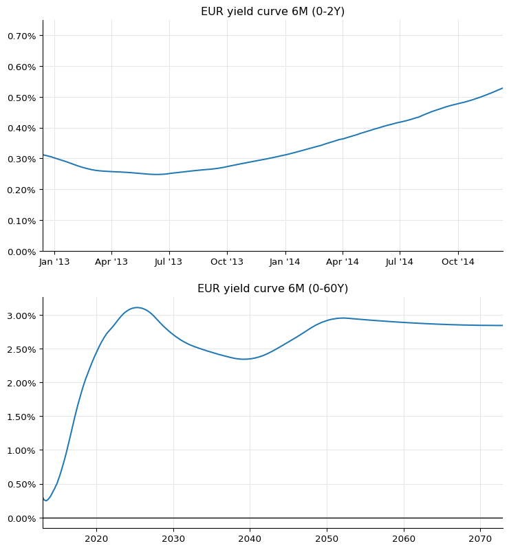
As for figure 32 in the paper, here’s how we can reproduce it:
fig = plt.figure(figsize=(9, 10))

spot = euribor6m_curve.referenceDate()
dates = [spot + ql.Period(i, ql.Weeks) for i in range(0, 2 * 52 + 1)]
rates = [
    euribor6m_curve.forwardRate(
        d, euribor6m.maturityDate(d), ql.Actual360(), ql.Simple
    ).rate()
    for d in dates
]

ax1 = fig.add_subplot(2, 1, 1)
ax1.set_title("EUR yield curve 6M (0-2Y)")
ax1.set_xlim(min(dates).to_date(), max(dates).to_date())
ax1.yaxis.set_major_formatter(PercentFormatter(1.0))
ax1.set_ylim(0.0, 0.0075)
ax1.plot_date([d.to_date() for d in dates], rates, "-")

spot = euribor6m_curve.referenceDate()
dates = [spot + ql.Period(i, ql.Months) for i in range(0, 60 * 12 + 1)]
rates = [
    euribor6m_curve.forwardRate(
        d, euribor6m.maturityDate(d), ql.Actual360(), ql.Simple
    ).rate()
    for d in dates
]

ax2 = fig.add_subplot(2, 1, 2)
ax2.set_title("EUR yield curve 6M (0-60Y)")
ax2.axhline(0.0, linewidth=1, color="black")
ax2.set_xlim(min(dates).to_date(), max(dates).to_date())
ax2.yaxis.set_major_formatter(PercentFormatter(1.0))
ax2.plot_date([d.to_date() for d in dates], rates, "-");
12-months Euribor curve
For the 12-months curve, we’ll use the data from figure 33 and reproduce figure 34.
we’ll start with the quoted 12-months deposit and 12x24 FRA (see figures 4 and 6).
euribor12m = ql.Euribor1Y()
helpers = [
    ql.DepositRateHelper(
        ql.QuoteHandle(ql.SimpleQuote(0.54 / 100)),
        ql.Period(12, ql.Months),
        2,
        ql.TARGET(),
        ql.Following,
        False,
        ql.Actual360(),
    )
]
helpers += [
    ql.FraRateHelper(
        ql.QuoteHandle(ql.SimpleQuote(0.5070 / 100)), 12, euribor12m
    )
]
Unfortunately, there are no quoted swap rates against 12-months Euribor. However, the market quotes 6- vs 12-months basis swaps; and more importantly, it quotes them as a portfolio of two IRS, payer and receiver, both accruing annual fixed coupons against Euribor 6M and 12M, respectively. The spread between the two fixed legs is quoted so that it sets the NPV of the portfolio at zero.
Given that the market also quotes the fair fixed rate for one of the two swaps, i.e., the one paying a fixed rate against Euribor 6M, it’s straightforward to see that the fair fixed rate for the swap against Euribor 12M can be obtained by just adding the 6M rate to the basis spread: that is, if the NPV of a swap $S_1$ paying $K$ against Euribor 6M is 0, and if the NPV of the portfolio of $S_1$ minus another swap $S_2$ paying $K+S$ against Euribor 12M is also 0, then the NPV of $S_2$ must be 0 as well.
This gives us quoted swap rates against Euribor 12M up to 30 years, which is the longest quoted maturity for basis swaps. The data are from figures 9 and 15.
helpers += [
    ql.SwapRateHelper(
        ql.QuoteHandle(ql.SimpleQuote((rate + basis) / 100)),
        ql.Period(tenor, ql.Years),
        ql.TARGET(),
        ql.Annual,
        ql.Unadjusted,
        ql.Thirty360(ql.Thirty360.BondBasis),
        euribor12m,
        ql.QuoteHandle(),
        ql.Period(0, ql.Days),
        discount_curve,
    )
    for rate, basis, tenor in [
        (0.424, 0.179, 3),
        (0.576, 0.164, 4),
        (0.762, 0.151, 5),
        (0.954, 0.139, 6),
        (1.135, 0.130, 7),
        (1.303, 0.123, 8),
        (1.452, 0.118, 9),
        (1.584, 0.113, 10),
        (1.809, 0.106, 12),
        (2.037, 0.093, 15),
        (2.187, 0.080, 20),
        (2.234, 0.072, 25),
        (2.256, 0.066, 30),
    ]
]
Again, we’ll be using synthetic helpers to improve the shape of the short end of the curve. The same procedure we used for the Euribor 6M curve lets us create deposits with a number of maturities below 1 year; I’ll skip the calculation and just create helpers with the the resulting rates as reported by the paper.
synth_helpers = [
    ql.DepositRateHelper(
        ql.QuoteHandle(ql.SimpleQuote(rate / 100)),
        ql.Period(*tenor),
        2,
        ql.TARGET(),
        ql.Following,
        False,
        ql.Actual360(),
    )
    for rate, tenor in [
        (0.6537, (1, ql.Months)),
        (0.6187, (3, ql.Months)),
        (0.5772, (6, ql.Months)),
        (0.5563, (9, ql.Months)),
    ]
]
It is also possible to build synthetic FRAs: their construction is explained in the paper. I’ll leave it, possibly, to a later version of this notebook; for the time being, I’ll just add the finished helpers.
synth_helpers += [
    ql.FraRateHelper(
        ql.QuoteHandle(ql.SimpleQuote(rate / 100)), months_to_start, euribor12m
    )
    for rate, months_to_start in [
        (0.4974, 3),
        (0.4783, 6),
        (0.4822, 9),
        (0.5481, 15),
        (0.6025, 18),
    ]
]
Finally, we can extend the long end of the curve by creating synthetic swaps with maturities above 30 years. To calculate their rates, we add the swap rates against Euribor 6M (quoted up to 60 years) to the last quoted basis spread.
last_basis = 0.066
synth_helpers += [
    ql.SwapRateHelper(
        ql.QuoteHandle(ql.SimpleQuote((rate + last_basis) / 100)),
        ql.Period(tenor, ql.Years),
        ql.TARGET(),
        ql.Annual,
        ql.Unadjusted,
        ql.Thirty360(ql.Thirty360.BondBasis),
        euribor12m,
        ql.QuoteHandle(),
        ql.Period(0, ql.Days),
        discount_curve,
    )
    for rate, tenor in [(2.295, 35), (2.348, 40), (2.421, 50), (2.463, 60)]
]
Bootstrapping over the whole set of real and synthetic quotes gives us our final Euribor 12M curve:
euribor12m_curve = ql.PiecewiseLogCubicDiscount(
    2, ql.TARGET(), helpers + synth_helpers, ql.Actual365Fixed()
)
euribor12m_curve.enableExtrapolation()
For comparison, we can build another one excluding the synthetic helpers. Note that this second curve won’t extend beyond 30 years.
euribor12m_curve_0 = ql.PiecewiseLogCubicDiscount(
    2, ql.TARGET(), helpers, ql.Actual365Fixed()
)
euribor12m_curve_0.enableExtrapolation()
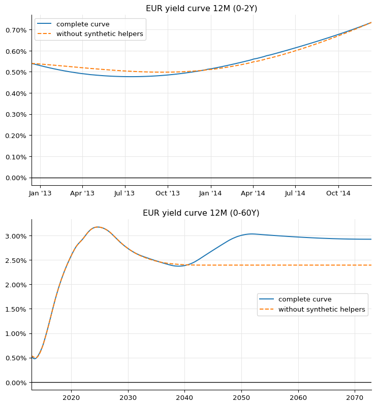
The two curves are plotted together in the two following graphs, which also reproduce figure 34 in the paper. The solid line corresponds to the complete curve, and the dashed line to the curve without the synthetic helpers. The differences are obvious, both in the short and in the long end.
fig = plt.figure(figsize=(9, 10))

spot = euribor12m_curve.referenceDate()
dates = [spot + ql.Period(i, ql.Weeks) for i in range(0, 2 * 52 + 1)]
rates_0 = [
    euribor12m_curve_0.forwardRate(
        d, euribor12m.maturityDate(d), ql.Actual360(), ql.Simple
    ).rate()
    for d in dates
]
rates = [
    euribor12m_curve.forwardRate(
        d, euribor12m.maturityDate(d), ql.Actual360(), ql.Simple
    ).rate()
    for d in dates
]

ax1 = fig.add_subplot(2, 1, 1)
ax1.set_title("EUR yield curve 12M (0-2Y)")
ax1.axhline(0.0, linewidth=1, color="black")
ax1.set_xlim(min(dates).to_date(), max(dates).to_date())
ax1.yaxis.set_major_formatter(PercentFormatter(1.0))
ax1.plot_date([d.to_date() for d in dates], rates, "-", label="complete curve")
ax1.plot_date(
    [d.to_date() for d in dates],
    rates_0,
    "--",
    label="without synthetic helpers",
)
ax1.legend()

dates = [spot + ql.Period(i, ql.Months) for i in range(0, 60 * 12 + 1)]
rates_0 = [
    euribor12m_curve_0.forwardRate(
        d, euribor12m.maturityDate(d), ql.Actual360(), ql.Simple
    ).rate()
    for d in dates
]
rates = [
    euribor12m_curve.forwardRate(
        d, euribor12m.maturityDate(d), ql.Actual360(), ql.Simple
    ).rate()
    for d in dates
]

ax2 = fig.add_subplot(2, 1, 2)
ax2.set_title("EUR yield curve 12M (0-60Y)")
ax2.axhline(0.0, linewidth=1, color="black")
ax2.set_xlim(min(dates).to_date(), max(dates).to_date())
ax2.yaxis.set_major_formatter(PercentFormatter(1.0))
ax2.plot_date([d.to_date() for d in dates], rates, "-", label="complete curve")
ax2.plot_date(
    [d.to_date() for d in dates],
    rates_0,
    "--",
    label="without synthetic helpers",
)
ax2.legend();
3-months Euribor curve
For the 3-months Euribor, we can use a strip of very liquid futures after the 3-months deposit; their rates, and those of other instruments used for this curve, are listed in figures 29.
euribor3m = ql.Euribor3M()
helpers = [
    ql.DepositRateHelper(
        ql.QuoteHandle(ql.SimpleQuote(0.179 / 100)),
        ql.Period(3, ql.Months),
        3,
        ql.TARGET(),
        ql.Following,
        False,
        ql.Actual360(),
    )
]
helpers += [
    ql.FuturesRateHelper(
        ql.QuoteHandle(ql.SimpleQuote(100 - rate)),
        start_date,
        euribor3m,
        ql.QuoteHandle(),
    )
    for rate, start_date in [
        (0.1775, ql.Date(19, ql.December, 2012)),
        (0.1274, ql.Date(20, ql.March, 2013)),
        (0.1222, ql.Date(19, ql.June, 2013)),
        (0.1269, ql.Date(18, ql.September, 2013)),
        (0.1565, ql.Date(18, ql.December, 2013)),
        (0.1961, ql.Date(19, ql.March, 2014)),
        (0.2556, ql.Date(18, ql.June, 2014)),
        (0.3101, ql.Date(17, ql.September, 2014)),
    ]
]
For the swaps, we combine quotes for the swaps against 6-months Euribor with quotes for the 3-months against 6-months basis swap, like we did for the 12-months curve; basis swap quotes for this tenor are available up to 50 years, as shown in figure 15. In this case, though, the fixed rate against Euribor 3M is lower than the one against Euribor 6M; therefore, the basis must be subtracted from the quoted rate:
helpers += [
    ql.SwapRateHelper(
        ql.QuoteHandle(ql.SimpleQuote((rate - basis) / 100)),
        ql.Period(tenor, ql.Years),
        ql.TARGET(),
        ql.Annual,
        ql.Unadjusted,
        ql.Thirty360(ql.Thirty360.BondBasis),
        euribor3m,
        ql.QuoteHandle(),
        ql.Period(0, ql.Days),
        discount_curve,
    )
    for rate, basis, tenor in [
        (0.424, 0.1395, 3),
        (0.576, 0.1390, 4),
        (0.762, 0.1395, 5),
        (0.954, 0.1375, 6),
        (1.135, 0.1350, 7),
        (1.303, 0.1320, 8),
        (1.452, 0.1285, 9),
        (1.584, 0.1250, 10),
        (1.809, 0.1170, 12),
        (2.037, 0.1045, 15),
        (2.187, 0.0885, 20),
        (2.234, 0.0780, 25),
        (2.256, 0.0700, 30),
        (2.348, 0.0600, 40),
        (2.421, 0.0540, 50),
    ]
]
Again, synthetic deposit rates can be calculated and added for short maturities…
synth_helpers = [
    ql.DepositRateHelper(
        ql.QuoteHandle(ql.SimpleQuote(rate / 100)),
        ql.Period(*tenor),
        2,
        ql.TARGET(),
        ql.Following,
        False,
        ql.Actual360(),
    )
    for rate, tenor in [
        (0.1865, (2, ql.Weeks)),
        (0.1969, (3, ql.Weeks)),
        (0.1951, (1, ql.Months)),
        (0.1874, (2, ql.Months)),
    ]
]
…and again, we can add a few synthetic swaps where quotes for the 3-months versus 6-months Euribor are not available. We can calculate a quote for the 35-years basis swap by interpolating between the 30- and 40-years quotes, and one for the 60-years swap by extrapolating the 50-years quote flatly, like we did for the 12-months Euribor. Note that in this case, the authors of the paper choose instead to extrapolate the previous quotes linearly; anyway, this gives a difference of less than half a basis point.
synth_helpers += [
    ql.SwapRateHelper(
        ql.QuoteHandle(ql.SimpleQuote((rate - basis) / 100)),
        ql.Period(tenor, ql.Years),
        ql.TARGET(),
        ql.Annual,
        ql.Unadjusted,
        ql.Thirty360(ql.Thirty360.BondBasis),
        euribor3m,
        ql.QuoteHandle(),
        ql.Period(0, ql.Days),
        discount_curve,
    )
    for rate, basis, tenor in [(2.295, 0.0650, 35), (2.463, 0.0540, 60)]
]
Turn of year
This is not the end of the story, though, since one of the futures we used turns out to be out of line with respect to the others in the strip.
futures = [
    (0.1775, ql.Date(19, ql.December, 2012)),
    (0.1274, ql.Date(20, ql.March, 2013)),
    (0.1222, ql.Date(19, ql.June, 2013)),
    (0.1269, ql.Date(18, ql.September, 2013)),
    (0.1565, ql.Date(18, ql.December, 2013)),
    (0.1961, ql.Date(19, ql.March, 2014)),
    (0.2556, ql.Date(18, ql.June, 2014)),
    (0.3101, ql.Date(17, ql.September, 2014)),
]
Not surprisingly, it’s the one that spans the end of the year and thus includes the corresponding jump; that is, the one at index 4 in the list, starting on December 18th. This can be seen clearly enough by fitting a spline between the other futures and plotting the quoted value against the curve:
spot = euribor6m_curve.referenceDate()
day_counter = euribor3m.dayCounter()
quotes, times = zip(
    *[(q, day_counter.yearFraction(spot, d)) for q, d in futures]
)
f = ql.MonotonicCubicNaturalSpline(
    times[:4] + times[5:], quotes[:4] + quotes[5:]
)
ts, fs = zip(*[(t, f(t, True)) for t in np.arange(0.0, 2.0, 0.01)])
ax = plt.figure(figsize=(9, 6)).add_subplot(1, 1, 1)
ax.yaxis.set_major_formatter(PercentFormatter(100.0))
ax.plot(ts, fs)
ax.plot(times, quotes, "o");
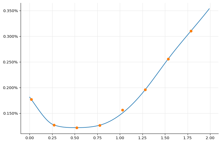
We can also ask the interpolation for the estimated value and compare it with the real one:
print(f"{quotes[4]:.3} %")
print(f"{f(times[4]):.3} %")
0.157 %
0.151 %
To account for the jump, we can estimate the corresponding discount factor $e^{-J*\tau}$ (where both $J$ and $\tau$ are calculated with respect to the tenor of the futures) and add it to the curve.
J = (quotes[4] - f(times[4])) / 100
tau = day_counter.yearFraction(
    ql.Date(18, ql.December, 2013), ql.Date(18, ql.March, 2014)
)
print(f"{J*100:.3} %")
print(tau)
0.00593 %
0.25
jumps = [ql.QuoteHandle(ql.SimpleQuote(math.exp(-J * tau)))]
jump_dates = [ql.Date(31, ql.December, 2013)]
euribor3m_curve = ql.PiecewiseLogCubicDiscount(
    2,
    ql.TARGET(),
    helpers + synth_helpers,
    ql.Actual365Fixed(),
    jumps,
    jump_dates,
)
euribor3m_curve.enableExtrapolation()
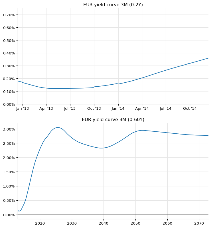
We can now reproduce figure 30 in the paper. The end-of-year jump can be seen clearly in the first plot.
fig = plt.figure(figsize=(9, 10))

spot = euribor3m_curve.referenceDate()
dates = [spot + ql.Period(i, ql.Weeks) for i in range(0, 2 * 52 + 1)]
rates = [
    euribor3m_curve.forwardRate(
        d, euribor3m.maturityDate(d), ql.Actual360(), ql.Simple
    ).rate()
    for d in dates
]

ax1 = fig.add_subplot(2, 1, 1)
ax1.set_title("EUR yield curve 3M (0-2Y)")
ax1.axhline(0.0, linewidth=1, color="black")
ax1.set_xlim(min(dates).to_date(), max(dates).to_date())
ax1.yaxis.set_major_formatter(PercentFormatter(1.0))
ax1.set_ylim(0.0, 0.0075)
ax1.plot_date([d.to_date() for d in dates], rates, "-")

dates = [spot + ql.Period(i, ql.Months) for i in range(0, 60 * 12 + 1)]
rates = [
    euribor3m_curve.forwardRate(
        d, euribor3m.maturityDate(d), ql.Actual360(), ql.Simple
    ).rate()
    for d in dates
]

ax2 = fig.add_subplot(2, 1, 2)
ax2.set_title("EUR yield curve 3M (0-60Y)")
ax2.axhline(0.0, linewidth=1, color="black")
ax2.set_xlim(min(dates).to_date(), max(dates).to_date())
ax2.yaxis.set_major_formatter(PercentFormatter(1.0))
ax2.plot_date([d.to_date() for d in dates], rates, "-");
1-month Euribor curve
Last, let’s bootstrap the 1-month Euribor curve. Quoted instruments based on this tenor include the 1-month deposit and interest-rate swaps paying a monthly fixed rate against 1-month Euribor with maturities up to 1 year; their rates are listed in figures 27.
euribor1m = ql.Euribor1M()
helpers = [
    ql.DepositRateHelper(
        ql.QuoteHandle(ql.SimpleQuote(0.110 / 100)),
        ql.Period(1, ql.Months),
        2,
        ql.TARGET(),
        ql.Following,
        False,
        ql.Actual360(),
    )
]
helpers += [
    ql.SwapRateHelper(
        ql.QuoteHandle(ql.SimpleQuote(rate / 100)),
        ql.Period(tenor, ql.Months),
        ql.TARGET(),
        ql.Monthly,
        ql.Unadjusted,
        ql.Thirty360(ql.Thirty360.BondBasis),
        euribor1m,
        ql.QuoteHandle(),
        ql.Period(0, ql.Days),
        discount_curve,
    )
    for rate, tenor in [
        (0.106, 2),
        (0.096, 3),
        (0.085, 4),
        (0.079, 5),
        (0.075, 6),
        (0.071, 7),
        (0.069, 8),
        (0.066, 9),
        (0.065, 10),
        (0.064, 11),
        (0.063, 12),
    ]
]
For longer maturities, we can combine the swaps against 6-months Euribor with the 1-month vs 6-months basis swaps shown in figure 15.
helpers += [
    ql.SwapRateHelper(
        ql.QuoteHandle(ql.SimpleQuote((rate - basis) / 100)),
        ql.Period(tenor, ql.Years),
        ql.TARGET(),
        ql.Annual,
        ql.Unadjusted,
        ql.Thirty360(ql.Thirty360.BondBasis),
        euribor1m,
        ql.QuoteHandle(),
        ql.Period(0, ql.Days),
        discount_curve,
    )
    for rate, basis, tenor in [
        (0.324, 0.226, 2),
        (0.424, 0.238, 3),
        (0.576, 0.246, 4),
        (0.762, 0.250, 5),
        (0.954, 0.250, 6),
        (1.135, 0.248, 7),
        (1.303, 0.245, 8),
        (1.452, 0.241, 9),
        (1.584, 0.237, 10),
        (1.703, 0.233, 11),
        (1.809, 0.228, 12),
        (2.037, 0.211, 15),
        (2.187, 0.189, 20),
        (2.234, 0.175, 25),
        (2.256, 0.163, 30),
    ]
]
As before, we can use synthetic deposits for maturities below the 1-month tenor…
synth_helpers = [
    ql.DepositRateHelper(
        ql.QuoteHandle(ql.SimpleQuote(rate / 100)),
        ql.Period(*tenor),
        2,
        ql.TARGET(),
        ql.Following,
        False,
        ql.Actual360(),
    )
    for rate, tenor in [
        (0.0661, (1, ql.Days)),
        (0.098, (1, ql.Weeks)),
        (0.0993, (2, ql.Weeks)),
        (0.1105, (3, ql.Weeks)),
    ]
]
…and we’ll extend the 30-years basis spread flatly to combine it with longer-maturity swaps against 6-months Euribor.
last_basis = 0.163
synth_helpers += [
    ql.SwapRateHelper(
        ql.QuoteHandle(ql.SimpleQuote((rate - last_basis) / 100)),
        ql.Period(tenor, ql.Years),
        ql.TARGET(),
        ql.Annual,
        ql.Unadjusted,
        ql.Thirty360(ql.Thirty360.BondBasis),
        euribor1m,
        ql.QuoteHandle(),
        ql.Period(0, ql.Days),
        discount_curve,
    )
    for rate, tenor in [(2.295, 35), (2.348, 40), (2.421, 50), (2.463, 60)]
]
This curve, too, shows a jump at the end of the year. The paper claims that it can be determined and corrected by interpolating the quoted swaps with maturities from 1 to 12 months, but I haven’t reproduced the calculation yet. For the time being, I’ll just use the value reported in the paper and calculate the corresponding discount factor.
J = 0.0016
t_j = euribor1m.dayCounter().yearFraction(
    ql.Date(31, ql.December, 2012), ql.Date(2, ql.January, 2013)
)
B = 1.0 / (1.0 + J * t_j)
jumps = [ql.QuoteHandle(ql.SimpleQuote(B))]
jump_dates = [ql.Date(31, ql.December, 2013)]
euribor1m_curve = ql.PiecewiseLogCubicDiscount(
    2,
    ql.TARGET(),
    helpers + synth_helpers,
    ql.Actual365Fixed(),
    jumps,
    jump_dates,
)
euribor1m_curve.enableExtrapolation()
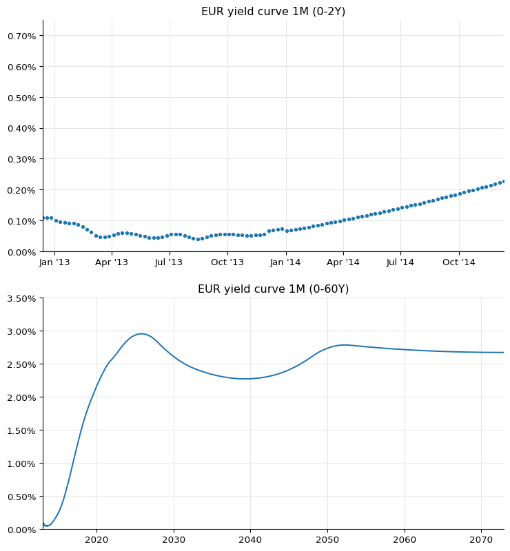
This last curve gives us figure 28 in the paper, down to the oscillations during the first year.
fig = plt.figure(figsize=(9, 10))

spot = euribor1m_curve.referenceDate()
dates = [spot + ql.Period(i, ql.Weeks) for i in range(0, 2 * 52 + 1)]
rates = [
    euribor1m_curve.forwardRate(
        d, euribor1m.maturityDate(d), ql.Actual360(), ql.Simple
    ).rate()
    for d in dates
]

ax1 = fig.add_subplot(2, 1, 1)
ax1.set_title("EUR yield curve 1M (0-2Y)")
ax1.axhline(0.0, linewidth=1, color="black")
ax1.set_xlim(min(dates).to_date(), max(dates).to_date())
ax1.yaxis.set_major_formatter(PercentFormatter(1.0))
ax1.set_ylim(0.0, 0.0075)
ax1.plot_date([d.to_date() for d in dates], rates, ".")

dates = [spot + ql.Period(i, ql.Months) for i in range(0, 60 * 12 + 1)]
rates = [
    euribor1m_curve.forwardRate(
        d, euribor1m.maturityDate(d), ql.Actual360(), ql.Simple
    ).rate()
    for d in dates
]

ax2 = fig.add_subplot(2, 1, 2)
ax2.set_title("EUR yield curve 1M (0-60Y)")
ax2.set_xlim(min(dates).to_date(), max(dates).to_date())
ax2.yaxis.set_major_formatter(PercentFormatter(1.0))
ax2.set_ylim(0.0, 0.035)
ax2.plot_date([d.to_date() for d in dates], rates, "-");
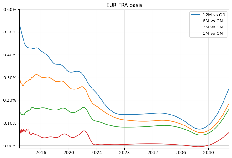
Basis curves
Finally, like the authors of the paper, we summarize the results by calculating the difference between the FRA rates calculated on the corresponding Euribor curve and those calculated on the ON curve. This lets us reproduce the top panel of figure 35, and ends this notebook.
dates = [spot + ql.Period(i, ql.Months) for i in range(0, 12 * 30 + 1)]


def basis(curve, tenor):
    results = []
    for d in dates:
        d2 = ql.TARGET().advance(d, ql.Period(*tenor), ql.ModifiedFollowing)
        FRA1 = curve.forwardRate(d, d2, ql.Actual360(), ql.Simple).rate()
        FRA2 = eonia_curve.forwardRate(d, d2, ql.Actual360(), ql.Simple).rate()
        results.append(FRA1 - FRA2)
    return results


basis_1m = basis(euribor1m_curve, (1, ql.Months))
basis_3m = basis(euribor3m_curve, (3, ql.Months))
basis_6m = basis(euribor6m_curve, (6, ql.Months))
basis_12m = basis(euribor12m_curve, (12, ql.Months))

ax = plt.figure(figsize=(9, 6)).add_subplot(1, 1, 1)
ax.set_title("EUR FRA basis")
ax.axhline(0.0, linewidth=1, color="black")
ax.set_xlim(min(dates).to_date(), max(dates).to_date())
ax.yaxis.set_major_formatter(PercentFormatter(1.0))
ax.set_ylim(-0.0001, 0.006)
ax.plot_date([d.to_date() for d in dates], basis_12m, "-", label="12M vs ON")
ax.plot_date([d.to_date() for d in dates], basis_6m, "-", label="6M vs ON")
ax.plot_date([d.to_date() for d in dates], basis_3m, "-", label="3M vs ON")
ax.plot_date([d.to_date() for d in dates], basis_1m, "-", label="1M vs ON")
ax.legend();