Using QuantLib interactively

Hello, dear reader.

Today’s post was originally published in the September 2023 issue of Wilmott Magazine. The full source file and the required data are available on my Tutorial page, together with code from other articles and, when available, either the articles themselves or corresponding blog posts like this one.

Subscribe to my Substack to receive my posts in your inbox, or follow me on Twitter or LinkedIn if you want to be notified of new posts, or subscribe via RSS if you’re the tech type: the buttons for all that are in the footer. Also, I’m available for training, both online and (when possible) on-site: visit my Training page for more information.

Using QuantLib interactively

Or, the joys of quick feedback

This time, I thought we could have a look specifically at why you would want to use QuantLib from Python. The advantages, besides a simpler syntax than, say, C++, are interactivity (no compile-link-run cycle) and the possibility to use the larger Python ecosystem; for instance, Jupyter, which provides a notebook-like environment where Python code can be mixed with descriptive text and with figures, usually generated by the code itself. It can be used for interactive data exploration and calculation, as well as for demonstrations: for instance, I published a series of videos on YouTube in which I use Jupyter notebooks to showcase QuantLib.

What are we looking at?

The code below is from another Jupyter notebook that I wrote, and shows how to use QuantLib to fit a credit curve to a set of bond prices. I used it, for instance, in a training I did for a team at a large and famous institution that will remain unnamed. Now, why am I telling you this? It’s not just for bragging rights, or to astutely hint at the fact that I’m indeed available for training teams. It’s because of something that happened during the training, and that I’m not going to spoil right now. A master of suspense, that’s what they call me. Onwards with the code!

Required modules

Not surprisingly, the first required module is QuantLib. The part of the library which is exported to Python is contained in a single module, due to the way we’re generating the wrapper code. The name is, of course, QuantLib; for convenience, I usually shorten it to ql following common Python practice. Hence, the line import QuantLib as ql that appears at the top of this code and of my other notebooks.

import QuantLib as ql
import csv
from matplotlib import pyplot as plt
from matplotlib.dates import YearLocator
from matplotlib.ticker import PercentFormatter


def new_plot():
    f = plt.figure(figsize=(8, 5))
    ax = f.add_subplot(1, 1, 1)

    ax.xaxis.grid(True, "major", color="lightgray")
    ax.yaxis.grid(True, "major", color="lightgray")
    ax.xaxis.set_major_locator(YearLocator(10))

    return f, ax

The other modules are the csv module from the Python standard library, used to read and write CSV files, and matplotlib, not a standard module but one of the modules most commonly used for plotting. I’m going to gloss over the details of the new_plot function that follows the import statements; when called, it creates a new, empty Matplotlib plot and configures its x and y grids. Its calling code will then add data to the returned plot.

Global evaluation date

today = ql.Date(21, ql.September, 2021)
ql.Settings.instance().evaluationDate = today

Not a lot to see here. As I mentioned in previous notebooks, QuantLib has a global evaluation date; here I’m setting it. A day may come when I show what happens when we change the evaluation date; but it is not this day.

Read bond data from a CSV file

This part of the code reads the data file shown in the box; each row corresponds to a bond and contains its start date, its maturity date, the coupon rate it pays, and a quoted price. For simplicity, all bonds will have the same frequency and day-count convention; but we might have specified those in this file, too.

def from_iso(date):
    return ql.Date(date, "%Y-%m-%d")


def apply_types(row):
    return [
        from_iso(row[0]),
        from_iso(row[1]),
        float(row[2]),
        float(row[3]),
    ]


with open("2023-09.csv") as f:
    reader = csv.reader(f)
    next(reader)  # skip header
    data = [apply_types(row) for row in reader]
data.sort(key=lambda r: r[1])

The csv module in the Python standard library helps with parsing and quotation (if any) but only reads strings and doesn’t try to infer types; therefore we need a couple of helper functions to read the data in the correct formats and types. The first, from_iso, converts a date written in ISO format into a QuantLib date object; other formats can be parsed as well, by specifying their format string. The second, apply_types, takes one row (parsed as a list of strings) and converts each element into the proper type. The final loop applies it to each row. We’re also sorting data by bond maturity; it’s not required for fitting, but it makes it easier to plot data.

Create bonds and helpers

Now we finally get into some QuantLib code; namely, we create the bonds that we’ll use for fitting the discount curve. For each row in the data, we create a coupon schedule based on the given start and maturity date (plus, as I mentioned, a few assumptions about the frequency, calendar and business-day convention; they might be in the data instead) and with the schedule, the corresponding coupon-paying bond. As we loop over the rows, we keep two lists: one contains the bonds themselves, and the other contains so-called bond helpers, which wrap the bonds and their quoted price and will be passed to the curve constructor as part of the objective function of the fit.

helpers = []
bonds = []
for start, maturity, coupon, price in data:
    schedule = ql.Schedule(
        start,
        maturity,
        ql.Period(1, ql.Years),
        ql.TARGET(),
        ql.ModifiedFollowing,
        ql.ModifiedFollowing,
        ql.DateGeneration.Backward,
        False,
    )
    bond = ql.FixedRateBond(
        3,
        100.0,
        schedule,
        [coupon / 100.0],
        ql.Actual360(),
        ql.ModifiedFollowing,
    )
    bonds.append(bond)
    helpers.append(ql.BondHelper(ql.QuoteHandle(ql.SimpleQuote(price)), bond))

Lastly, we create a pricing engine and set it to all bonds; once we have a fitted discount curve, we’ll pass it to its handle, now still empty, and use it to check the resulting bond prices.

discount_curve = ql.RelinkableYieldTermStructureHandle()
bond_engine = ql.DiscountingBondEngine(discount_curve)
for b in bonds:
    b.setPricingEngine(bond_engine)

Fit to a few curve models

The library implements a few parametric models such as Nelson-Siegel; in this example we’ll also use exponential splines, cubic B splines, and Svensson. The models are stored in a Python dictionary so that they can be easily retrieved based on a tag. A couple of them take parameters, but you’ll forgive me if I ignore them for brevity; they are documented in the library.

methods = {
    "Nelson/Siegel": ql.NelsonSiegelFitting(),
    "Exp. splines": ql.ExponentialSplinesFitting(True),
    "B splines": ql.CubicBSplinesFitting(
        [
            -30.0,
            -20.0,
            0.0,
            5.0,
            10.0,
            15.0,
            20.0,
            25.0,
            30.0,
            40.0,
            50.0,
        ],
        True,
    ),
    "Svensson": ql.SvenssonFitting(),
}

The fitting is performed by the FittedBondDiscountCurve class, which takes a list of bond helpers and the parametric model to calibrate, plus a few other parameters. As I mentioned, each bond helper contains a bond and its quoted price; the fitting process iterates over candidate values for the model parameters, reprices each of the bonds based on the resulting discount factors, and tries to minimize the difference between the resulting prices and the passed quotes.

tolerance = 1e-8
max_iterations = 5000
day_count = ql.Actual360()

curves = {
    tag: ql.FittedBondDiscountCurve(
        today,
        helpers,
        day_count,
        methods[tag],
        tolerance,
        max_iterations,
    )
    for tag in methods
}

Plot the curves

And now, we start to use to our advantage the plotting capabilities of Matplotlib. Together with the interactivity of the notebook, this gives us an environment where we can try out things, visualize data, and receive immediate feedback. For instance, the next bit of code plots the curves we just fitted; it creates a new plot, defines a set of monthly dates starting from today and spanning the next 30 years, and for each of the curves it extracts and plots the corresponding zero rates.

f, ax = new_plot()
ax.yaxis.set_major_formatter(PercentFormatter(1.0))
styles = iter(["-", "--", ":", "-."])

dates = [today + ql.Period(i, ql.Months) for i in range(12 * 30 + 1)]

for tag in curves:
    rates = [
        curves[tag].zeroRate(d, day_count, ql.Continuous).rate() for d in dates
    ]
    ax.plot_date(
        [d.to_date() for d in dates],
        rates,
        next(styles),
        label=tag,
    )
ax.legend(loc="best");

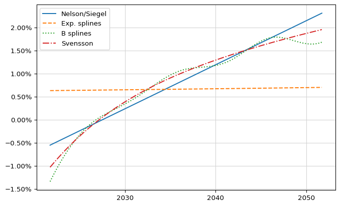
The figure above shows the result. The curves are a diverse bunch, to say the least: Nelson-Siegel and Svensson look sensible; exponential splines are almost flat and, compared to the others, look like the fit failed and we got some best-effort result; and cubic B splines are too wavy for my tastes. How can we get a better sense of their quality?

Plot the prices

With more visualization, of course. The quoted prices can be read from the data; they’re the last column. The bond prices implied by any of the curves are also not hard to get—do you remember we created a discount engine and set it to each bond? This pays off now: we can link its discount handle to the desired curve and ask each bond for its price; that’s what the prices function does. The error function calls the latter and returns the difference between calculated and quoted prices.

quoted_prices = [row[-1] for row in data]


def prices(tag):
    discount_curve.linkTo(curves[tag])
    return [b.cleanPrice() for b in bonds]


def errors(tag):
    return [q - p for p, q in zip(prices(tag), quoted_prices)]

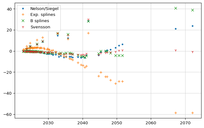
The bit of code that follows the functions plots the errors for each curve as function of the bond maturities. As you might have expected from the previous figure, Nelson-Siegel and Svensson yield smaller errors. Of the two, Svensson looks better in general but especially at longer maturities.

f, ax = new_plot()
maturities = [r[1].to_date() for r in data]
markers = iter([".", "+", "x", "1"])
for tag in curves:
    ax.plot_date(
        maturities,
        errors(tag),
        next(markers),
        label=tag,
    )
ax.legend(loc="best");

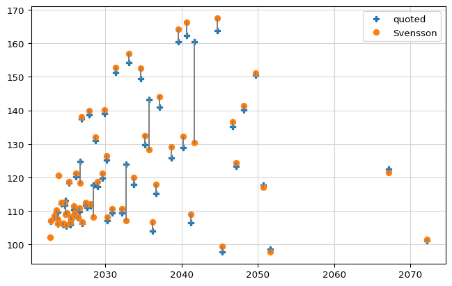
If we restrict ourselves to just one curve (let’s single out Svensson here as the best candidate) we can visualize the calibration errors in yet another way; that’s what the next plot does. Instead of the errors, it plots both quoted and calculated prices against maturities. The figure shows a fit which is not great overall, with noticeable errors for most bonds and a few much larger errors that don’t seem to follow any particular pattern.

f, ax = new_plot()
ps = prices("Svensson")
qs = quoted_prices
ax.plot_date(maturities, qs, "P", label="quoted")
ax.plot_date(maturities, ps, "o", label="Svensson")
ax.legend(loc="best")
for m, p, q in zip(maturities, ps, qs):
    ax.plot_date([m, m], [p, q], "-", color="grey")

Another point of view

So, what happened during the training I mentioned? It’s not unusual that, while I bring to the table my inside knowledge about QuantLib, the other people in the room are better quants. And when people with different expertise get together, good things usually happen. This time, one of the trainees said what you, too, might be thinking: “we should probably look at yields.”

And, thanks to Python and Jupyter, it took all of two minutes to visualize them. The yield corresponding to a quoted price can be calculated by passing it to the bondYield method of the corresponding bond; and after linking the desired discount curve, calling the same method without a target price will return the yield corresponding to the calculated price (the method is called simply yield in C++, but that’s a reserved keyword in Python, so we had to rename it while we export it.)

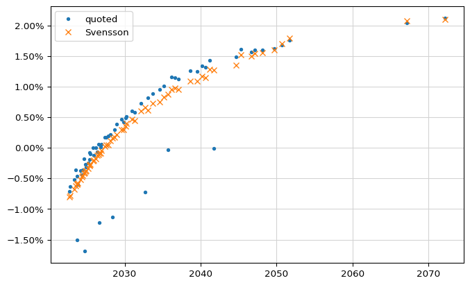
The result was enlightening. Most of the yields were on some kind of curve, but we had a few obvious outliers and they were pulling the fit away from the rest of the bonds.

quoted_yields = [
    b.bondYield(p, day_count, ql.Compounded, ql.Annual)
    for b, p in zip(bonds, quoted_prices)
]


def yields(tag):
    discount_curve.linkTo(curves[tag])
    return [b.bondYield(day_count, ql.Compounded, ql.Annual) for b in bonds]


f, ax = new_plot()
ax.yaxis.set_major_formatter(PercentFormatter(1.0))
ys = yields("Svensson")
qys = quoted_yields
ax.plot_date(maturities, qys, ".", label="quoted")
ax.plot_date(maturities, ys, "x", label="Svensson")
ax.legend(loc="best");

Remove outliers

Fortunately, it was also easy to improve the fit. Given the yields we calculated, we filtered out the helpers whose calculated yield differed by more than 50 basis points from the yield implied by the quoted price. We then created a new curve, passing only the filtered helpers.

ys = yields("Svensson")
qys = quoted_yields

filtered_helpers = [
    h for h, y1, y2 in zip(helpers, ys, qys) if abs(y1 - y2) < 0.005
]

curves["Svensson (new)"] = ql.FittedBondDiscountCurve(
    today,
    filtered_helpers,
    day_count,
    ql.SvenssonFitting(),
    tolerance,
    max_iterations,
)

Improved results

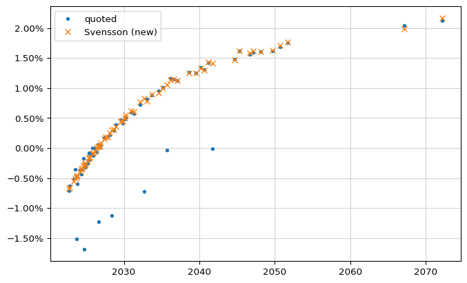
Again, it took almost no time to see the results. The rest of the code recreates the plots for yields…

f, ax = new_plot()
ax.yaxis.set_major_formatter(PercentFormatter(1.0))
ys = yields("Svensson")
ys2 = yields("Svensson (new)")
qys = quoted_yields
ax.plot_date(maturities, qys, ".", label="quoted")
ax.plot_date(maturities, ys2, "x", label="Svensson (new)")
ax.legend(loc="best");

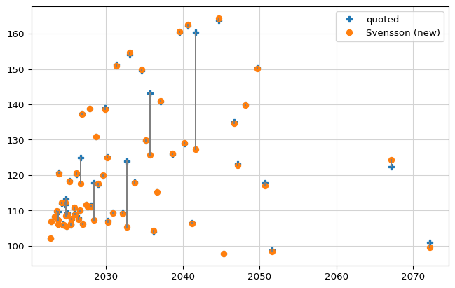
…and prices; both show a definite improvement of the quality of the fit. The mood of everyone involved in that session was also markedly improved.

f, ax = new_plot()
ps = prices("Svensson (new)")
qs = quoted_prices
ax.plot_date(maturities, qs, "P", label="quoted")
ax.plot_date(maturities, ps, "o", label="Svensson (new)")
ax.legend(loc="best")
for m, p, q in zip(maturities, ps, qs):
    ax.plot_date([m, m], [p, q], "-", color="grey")

Do you want to try?

To summarize: this kind of fast feedback and interactivity is the reason why, during these last years, using QuantLib in Python has become my go-to choice for exploration and troubleshooting. I hope this article will inspire you to give it a try; if you want to jump right into it without local installations, you can do it from your browser.

Go to the QuantLib-SWIG repository on GitHub (the home of the Python, Java, C# and R wrappers for QuantLib) and under the list of files you’ll see a README file, with a row of colorful badges displayed after the title. Click on the one that says “launch binder”, wait until the environment is built (it might take a while; the binder project has limited funds and resources and is looking for sponsors) and you’ll find yourself connected to a running Jupyter instance with a number of QuantLib examples that you can run and modify. You might have to right-click on the examples and select “Open with notebook” to get the runnable version.

Have fun, and see you next time!