Chapter 8, part 5 of n: finite-difference models
Welcome back, everybody.
This week, the next part of the series on the finite-difference framework.
But first, a small personal milestone: while I was in vacation, the 100th copy of Implementing QuantLib was sold on Leanpub. So, to the 100th reader who bought it between last Friday and Saturday, but also to all the others: thank you.
A couple of weeks ago we also had… well, actually, I don’t know if we had some kind of event or not. One morning I found in my inbox a few hundreds notifications that email addresses were removed from the QuantLib mailing lists. This usually happens when an address bounces a few times; the mailing-list software then flags it as obsolete and removes it. However, we never had that many at once. I’m not sure if this is some kind of glitch after the recent Sourceforge outages, or the result of their changing some kind of threshold. In any case, if you haven’t received emails from the list in a while, please check that you’re still subscribed. You can do so from http://quantlib.org/mailinglists.shtml: follow the “Subscribe/Unsubscribe/Preferences” link for the lists you’re subscribed to.
In the “back to business” department: there’s a few things happening in October. If you’re going to the WBS Fixed Income Conference in Paris, you may find me there. On Wednesday 7trh, I’ll be in the bench during Alexander Sokol’s workshop on how to add AAD to QuantLib (I’m listed as a presenter, but I’ll be just there ready to intervene if bits of particular QuantLib knowledge are needed). On the morning of Friday 9th, instead, I’ll have a slot to present QuantLib and its next developments in fixed income.
Also in October, I’ll be running my next Introduction to QuantLib Development course (in London, from Monday 19th to Wednesday 21st). Details and a registration form are at http://bit.ly/quantlib2015; you can also check out the hangout I did with Jacob Bettany to talk about it.
Follow me on Twitter if you want to be notified of new posts, or add me to your Google+ circles, or subscribe via RSS: the buttons for that are in the footer. Also, make sure to check my Training page.
The FiniteDifferenceModel class
The FiniteDifferenceModel class, shown in the next listing, uses an
evolution scheme to roll an asset back from a later time \( t_1 \)
to an earlier time \( t_2 \), taking into account any conditions we
add to the model and stopping at any time we declare as mandatory
(because something is supposed to happen at that point).
A word of warning: as I write this, I’m looking at this class after quite a few years and I realize that some things might have been done differently—not necessarily better, mind you, but there might be alternatives. After all this time, I can only guess at the reasons for such choices. While I describe the class, I’ll point out the alternatives and write my guesses.
    template<class Evolver>
    class FiniteDifferenceModel {
      public:
        typedef typename Evolver::traits traits;
        typedef typename traits::operator_type operator_type;
        typedef typename traits::array_type array_type;
        typedef typename traits::bc_set bc_set;
        typedef typename traits::condition_type condition_type;

        FiniteDifferenceModel(
            const Evolver& evolver,
            const std::vector<Time>& stoppingTimes =
                                          std::vector<Time>());

        FiniteDifferenceModel(
            const operator_type& L,
            const bc_set& bcs,
            const std::vector<Time>& stoppingTimes =
                                          std::vector<Time>());
        const Evolver& evolver() const{ return evolver_; }
        void rollback(array_type& a,
                      Time from,
                      Time to,
                      Size steps) {
             rollbackImpl(a,from,to,steps,
                          (const condition_type*) 0);
        }
        void rollback(array_type& a,
                      Time from,
                      Time to,
                      Size steps,
                      const condition_type& condition) {
            rollbackImpl(a,from,to,steps,&condition);
        }
      private:
        void rollbackImpl(array_type& a,
                          Time from,
                          Time to,
                          Size steps,
                          const condition_type* condition);
        Evolver evolver_;
        std::vector<Time> stoppingTimes_;
    };
I’ll just mention quickly that the class takes the evolution scheme as a template argument (as in the code, I might call it evolver for brevity from now on) and extracts some types from it via traits; that’s a technique you saw a few times already in earlier chapters.
So, first of all: the constructors. As you see, there’s two of them. One, as you’d expect, takes an instance of the evolution scheme and a vector of stopping times (and, not surprisingly, stores copies of them). The second, instead, takes the raw ingredients and builds the evolver.
The reason for the second one might have been convenience, that is, to avoid writing the slighly redundant
FiniteDifferenceModel<SomeScheme>(SomeScheme(L, bcs), ts);but I’m not sure that the convenience offsets having more code to
maintain (which, by the way, only works for some evolvers and not for
others; for instance, the base MixedScheme class doesn’t have a
constructor taking two arguments). This constructor might make more
sense when using one of the typedefs provided by the library, such as
StandardFiniteDifferenceModel, which hides the particular scheme
used; but I’d argue that you should know what scheme you’re using
anyway, since they have different requirements in terms of grid
spacing and time steps. (By the same argument, the
StandardFiniteDifferenceModel typedef would be a suggestion of what
scheme to use instead of a way to hide it.)
The main logic of the class is coded in the rollback and
rollbackImpl methods. The rollback method is the public interface
and has two overloaded signatures: one takes the array of values to
roll back, the initial and final times, and the number of steps to
use, while the other also takes a StepCondition instance to use at
each step. Both forward the call to the rollbackImpl method, which
takes a raw pointer to step condition as its last argument; the
pointer is null in the first case and contains the address of the
condition in the second.
Now, this is somewhat unusual in the library: in most other cases,
we’d just have a single public interface taking a shared_ptr and
defining a null default value. I’m guessing that this arrangement was
made to allow client code to simply create the step condition on the
stack and pass it to the method, instead of going through the motions
of creating a shared pointer (which, in fact, only makes sense if it’s
going to be shared; not passed, used and forgotten). Oh, and by the
way, the use of a raw pointer in the private interface doesn’t
contradict the ubiquitous use of smart pointers everywhere in the
library. We’re not allocating a raw pointer here; we’re just passing
the address of an object living on the stack (or inside a smart
pointer, for that matters) and which can manage its lifetime very
well, thank you.
One last remark on the interface: we’re treating boundary conditions
and step conditions differently, since the former are passed to the
constructor of the model and the latter are passed to the rollback
method. (Another difference is that we’re using explicit sets of
boundary conditions but just one step condition, which can be a
composite of several ones if needed. I have no idea why.) One reason
could have been that this allows more easily to use different step
conditions in different calls to rollback, that is, at different
times; but that could be done inside the step condition itself, as it
is passed the current time. The real generalization would have been to
pass the boundary conditions to rollback, too, as it’s currently not
possible to change them at a given time in the calculation. This would
have meant changing the interfaces of the evolvers, too: the boundary
conditions should have been passed to their step method, instead of
their constructors.
And finally, the implementation.
    void FiniteDifferenceModel::rollbackImpl(
                               array_type& a,
                               Time from,
                               Time to,
                               Size steps,
                               const condition_type* condition) {
        Time dt = (from-to)/steps, t = from;
        evolver_.setStep(dt);
        if (!stoppingTimes_.empty() && stoppingTimes_.back()==from) {
            if (condition)
                condition->applyTo(a,from);
        }
        for (Size i=0; i<steps; ++i, t -= dt) {
            Time now = t, next = t-dt;
            if (std::fabs(to-next) < std::sqrt(QL_EPSILON))
                next = to;
            bool hit = false;
            for (Integer j = stoppingTimes_.size()-1; j >= 0 ; --j) {
                if (next <= stoppingTimes_[j]
                         && stoppingTimes_[j] < now) {
                    hit = true;
                    evolver_.setStep(now-stoppingTimes_[j]);
                    evolver_.step(a,now);
                    if (condition)
                        condition->applyTo(a,stoppingTimes_[j]);
                    now = stoppingTimes_[j];
                }
            }
            if (hit) {
                if (now > next) {
                    evolver_.setStep(now - next);
                    evolver_.step(a,now);
                    if (condition)
                        condition->applyTo(a,next);
                }
                evolver_.setStep(dt);
            } else {
                evolver_.step(a,now);
                if (condition)
                    condition->applyTo(a, next);
            }
        }
    }
We’re going back from a later time from to an earlier time to in a
given number of steps. This gives us a length dt for each step,
which is set as the time step for the evolver. If from itself is a
stopping time, we also apply the step condition (if one was passed;
this goes for all further applications). Then we start going back step
by step, each time going from the current time t to the next time,
t-dt; we’ll also take care that the last time is actually to and
possibly snap it back to the correct value, because floating-point
calculations might have got us almost there but not quite.
If there were no stopping times to hit, the implementation would be
quite simple; in fact, the whole body of the loop would be the three
lines inside the very last else clause:
    evolver_.step(a,now);
    if (condition)
        condition->applyTo(a, next);
that is, we’d tell the evolver to roll back the values one step from
now, and we’d possibly apply the condition at the target time
next. This is what actually happens when there are no stopping times
between now and next, so that the control variable hit remains
false.
In case there are one or more stopping times in the middle of the step, things get a bit more complicated. Have a look at the upper half of the following figure, where I sketched a series of regular steps with two stopping times, \( s_1 \) and \( s_2 \), falling in the middle of two of them.
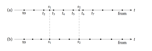
Let’s say we have just made the step from \( t_7 \) to \( t_6 \)
as described in the previous paragraph, and should now go back to \(
t_5 \). However, the code will detect that it should stop at \( s_2
\), which is between now and next; therefore, it will set the
control variable hit to true, it will set the step of the evolver to
the smaller step \( t_6-s_2 \) that will bring it to the stopping
time, and will perform the step (again, applying the condition
afterwards). Another, similar change of step would happen if there
were two or more stopping times in a single step; the code would then
step from one to the other. Finally, the code will enter the if
(hit) clause, which get things back to normal: it performs the
remaining step \( s_2-t_5 \) and then resets the step of the evolver
to the default value, so that it’s ready for the next regular step to
\( t_4 \).
As a final remark, let’s go back to trees for a minute. Talking about
the tree framework, I mentioned in
passing that the time grid of a lattice is built to include the
mandatory stopping times. In this case, the grid would have been the
one shown in the lower half of the previous figure. As you see, the
stopping times \( s_1 \) and \( s_2 \) were made part of the grid
by using slightly smaller steps between to and \( s_1 \) and
slightly larger steps between \( s_2 \) and from. (In this case,
the change results in the same number of steps as the
finite-difference grid. This is not always guaranteed; the tree grid
might end up having a couple of steps more or less than the requested
number.) I’m not aware of drawbacks in using either of the two
methods, but experts might disagree so I’m ready to stand
corrected. In any case, should you want to replicate the tree grid in
a finite-difference model, you can do so by making several calls to
rollback and going explicitly from stopping time to stopping time.