Chapter 8, part 10: basic finite-difference operators
Greetings.
This week, the fourth post in a series on the new finite-difference framework. If you’re one of those people that prefer binge reading, the first post is here. Unless you’re watching the whole first season of Luke Cage on Netflix, that is.
In other news, Hacktoberfest 2016 has begun, in which you can contribute to QuantLib (or any other project on GitHub) and earn a t-shirt. I didn’t get one last year, since I would have felt a bit like cheating if I had opened pull requests on QuantLib. What can I say? I’m old-fashioned. However, you shouldn’t have such qualms, so code away. (And I have a couple of projects to which I’ll try to contribute, too, so I might get a t-shirt after all. And you might hear shortly about one of them…)
Follow me on Twitter if you want to be notified of new posts, or add me to your Google+ circles, or subscribe via RSS: the buttons for that are in the footer. Also, make sure to check my Training page.
Basic operators
And now, some operators. As for the old framework, the most basic would be those that represent the first and second derivative along one of the axes. In this case, “basic” doesn’t necessarily mean “simple”; the formula for a three-point first derivative when the grid \( {x_1, \ldots, x_i, \ldots, x_N} \) is not equally spaced is
\[\frac{\partial f}{\partial x}(x_i) \approx -\frac{h_+}{h_-(h_- + h_+)} f(x_{i-1}) +\frac{h_+ - h_-}{h_+ h_-} f(x_i) +\frac{h_-}{h_+(h_- + h_+)} f(x_{i+1})\]where \( h_- = x_i - x_{i-1} \) and \( h_+ = x_{i+1} - x_i \), and the formula for the second derivative is just as long (if you’re interested, you can find the derivation of the formulas in Bowen and Smith [1]; preprints of the paper are available on the web). Furthermore, even though I’ve used the notation \( x_i \) to denote the \( i \)-th point along the relevant dimension, the points \( x_{i-1} \), \( x_i \) and \( x_{i+1} \) in the formula might actually be \( x_{i,j,k-1,l} \), \( x_{i,j,k,l} \) and \( x_{i,j,k+1,l} \) if we’re using a multi-dimensional array.
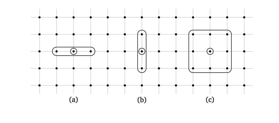
In any case, we’ll be using a three-point stencil such as the ones
shown for two different directions in cases (a) and (b) of the figure
below. Thus, both first- and second-derivative operators can be represented
as instantiations of the same underlying class, called
TripleBandLinearOp.
The basic definition of triple-band operators is similar to that of tridiagonal ones, which you might remember from a previous post. In that case, when applying the operator \( T \) to an array \( x \), the \( i \)-th element of the result \( y \) could be written as:
\[y_i = l_i x_{i-1} + d_i x_i + u_i x_{i+1}\]that is, a linear combination of the \( i \)-th element of \( x \) and of its two neighbors (\( l \), \( d \) and \( u \) are the lower diagonal, diagonal and upper diagonal). The triple-band operator generalizes the idea to multiple dimensions; here we have, for instance, that the element with indices \( i,j,k,l \) in the result is
\[y_{i,j,k,l} = l_k x_{i,j,k-1,l} + d_k x_{i,j,k,l} + u_k x_{i,j,k+1,l}\]which is still the combination of the element at the same place in the input and of its two neighbors in a given direction, which is the same for all elements. (I’m glossing over the elements at the boundaries, but those are easily managed by ignoring their non-existent neighbors.)
When the input and result array are flattened, and thus the operator is written as a 2-dimensional matrix, we find the three bands that give the operator its name. Let’s refer again to the figure above, and assume that the horizontal direction is the first and the vertical direction is the second, and therefore that the elements are enumerated first left to right and then top to bottom. In case (a), the two neighbors are close to the center point in the flattened array, and the operator turns out to be tridiagonal; in case (b), the neighbors are separated by a whole row of elements in the flattened array and the operator has two non-null bands away from the diagonal (which is also not null).
The interface of the TripleBandLinearOp class is shown in the
following listing.
class TripleBandLinearOp : public FdmLinearOp {
  public:
    TripleBandLinearOp(Size direction,
                       const shared_ptr<FdmMesher>& mesher);

    Array apply(const Array& r) const;
    Array solve_splitting(const Array& r, Real a,
                          Real b = 1.0) const;

    TripleBandLinearOp mult(const Array& u) const;
    TripleBandLinearOp multR(const Array& u) const;
    TripleBandLinearOp add(const TripleBandLinearOp& m) const;
    TripleBandLinearOp add(const Array& u) const;

    void axpyb(const Array& a, const TripleBandLinearOp& x,
               const TripleBandLinearOp& y, const Array& b);
  protected:
    TripleBandLinearOp() {}
    Size direction_;
    shared_array<Size> i0_, i2_;
    shared_array<Size> reverseIndex_;
    shared_array<Real> lower_, diag_, upper_;
    shared_ptr<FdmMesher> mesher_;
};
It contains a few methods besides the required apply. The
solve_splitting method, like the solveFor method in the interface
of old-style operators, is used to solve linear systems in which the
operator multiplies an array of unknowns, and thus enables to write
code using implicit schemes (which are usually stabler or faster than
explicit schemes using apply); and other methods such as mult or
add define a few operations that make it possible to perform basic
algebra and to build operators based on existing pieces (I’ll leave it
to you to check the code and see what’s what).
The constructor performs quite a bit of preliminary computations in order to make the operator ready to use.
TripleBandLinearOp::TripleBandLinearOp(
            Size direction,
            const shared_ptr<FdmMesher>& mesher) : /* ... */ {

   shared_ptr<FdmLinearOpLayout> layout = mesher->layout();
   vector<Size> newDim(layout->dim());
   iter_swap(newDim.begin(), newDim.begin()+direction_);
   vector<Size> newSpacing = FdmLinearOpLayout(newDim).spacing();
   iter_swap(newSpacing.begin(), newSpacing.begin()+direction_);

   for (FdmLinearOpIterator iter = layout->begin();
                            iter != layout->end(); ++iter) {
       const Size i = iter.index();
       i0_[i] = layout->neighbourhood(iter, direction, -1);
       i2_[i] = layout->neighbourhood(iter, direction,  1);
       const vector<Size>& coordinates = iter.coordinates();
       const Size newIndex =
           inner_product(coordinates.begin(), coordinates.end(),
                         newSpacing.begin(), Size(0));
       reverseIndex_[newIndex] = i;
   }
}
On the one hand, for each point in the layout, it stores in the two
arrays i0_ and i2_ the flattened indices of the two neighbors in
the given direction; this is done by means of the two calls to
layout->neighborhood, and allows the core of the apply method to
be written as a simple loop similar to:
for (Size i=0; i < layout->size(); ++i) {
    result[i] =
        lower_[i]*a[i0_[i]] + diag_[i]*a[i] + upper_[i]*a[i2_[i]];
}
where a is the array to which the operator is applied, and which
translates into code the equation I wrote above for \( y_{i,j,k,l} \).
(As a side note, the loop in the apply method would seem like an
obvious candidate for parallelization, and in fact we tried to speed
it up by adding a #pragma omp parallel for. However, this didn’t
seem to make the code any faster, and in some cases it actually hurt
performance. It might be that the compiler is using parallel
instructions already and making a better job when left alone. I’m an
absolute beginner at this, though, so I’ll leave it to you to
investigate the matter if you’re interested.)
On the other hand, the constructor fills the reverseIndex_ array,
which provides support for the implementation of solve_splitting.
In short, and oversimplifying a bit, the algorithm used for solving
the system is the same used for tridiagonal operators and involves a
double sweep of the array that yields the result in linear time.
However, the algorithm is required to sweep the array in the correct
order, that is, along the direction of the derivative. Referring
again to the figure, looping over the usual flattened index would
sweep the array horizontally, and therefore would only work in case
(a) but not in case (b).
The code solves this by introducing a second flattened index. Let’s
say we have a four-dimensional array with indices \( i,j,k,l \) and
corresponding sizes \( M,N,P,Q \), and that we want to take the
derivative along the \( k \) index. The spacing of the layout is
\( (1, M, MN, MNP) \), so the triple \( (i,j,k,l) \) yields the
flattened index \( I = i+M\cdot j + MN\cdot k + MNP\cdot l \). Now,
what the constructor does is to create a new spacing with its first
dimension swapped with the one corresponding to the derivative; in
this example, it would be \( (MN, M, 1, MNP) \). This defines a new
flattened index \( \tilde{I} = MN\cdot i + M\cdot j + k + MNP\cdot l
\) that sweeps the array so that consecutive values of \( \tilde{I}
\) map to adjacent elements in the \( k \) direction. Finally, the
values of \( I \) corresponding to each \( \tilde{I} \) are saved
in the reverseIndex_ array.
This allows the solve_splitting method to perform it work
correctly. The two loop will enumerate all the values of \( \tilde{I}
\) in order, and thus will sweep the array in the correct direction;
and the reverseIndex_ array will give us the corresponding ordinary
index that can be used to access the elements into the passed array.
Array TripleBandLinearOp::solve_splitting(const Array& r,
                                          Real a, Real b) const {
    // ... initializations ...
    Size rim1 = reverseIndex_[0];
    Real bet=1.0/(a*diag_[rim1]+b);
    retVal[reverseIndex_[0]] = r[rim1]*bet;
    for (Size j=1; j<=layout->size()-1; j++){
        const Size ri = reverseIndex_[j];
        tmp[j] = a*upper_[rim1]*bet;
        bet=1.0/(b+a*(diag_[ri]-tmp[j]*lower_[ri]));
        retVal[ri] = (r[ri]-a*lower_[ri]*retVal[rim1])*bet;
        rim1 = ri;
    }
    for (Size j=layout->size()-2; j>0; --j)
        retVal[reverseIndex_[j]] -=
                tmp[j+1]*retVal[reverseIndex_[j+1]];
    retVal[reverseIndex_[0]] -= tmp[1]*retVal[reverseIndex_[1]];

    return retVal;
}
Based on TripleBandLinearOp, the framework defines generic operators
for the first and second derivative along a given direction; they are
sketched in the listing that follows. As you see, they’re simple
enough: they only declare the constructor, which fills the lower_,
diag_ and upper_ arrays with the correct values (for instance, the
coefficients of \( f(x_{i-1}) \), \( f(x_i) \) and \( f(x_{i+1})
\) in the equation for \( \frac{\partial f}{\partial x}(x_i) \))
based on the passed layout.
class FirstDerivativeOp : public TripleBandLinearOp {
  public:
    FirstDerivativeOp(Size direction,
                      const shared_ptr<FdmMesher>& mesher);
};

class SecondDerivativeOp : public TripleBandLinearOp {
  public:
    SecondDerivativeOp(Size direction,
                       const shared_ptr<FdmMesher>& mesher);
};
To round up the basic operators, I’ll just mention that the framework
also defines a NinePointLinearOp class, managing stencils like the
one in case (c) of the figure above, and its derived class
SecondOrderMixedDerivativeOp, modeling the cross-derivative \(
\frac{\partial^2 f}{\partial x_i \partial x_j} \) along two
directions.
In next post: an example or two of real-world operators.
Bibliography
[1] M. K. Bowen and R. Smith, Derivative formulae and errors for non-uniformly spaced points. In Proceedings of the Royal Society of London A: Mathematical, Physical and Engineering Sciences, volume 461, pages 1975–1997. The Royal Society, 2005.